Welcome to METEO 410
Welcome to METEO 410Quick Facts about METEO 410
METEO 410 is the capstone course in Penn State's online program that confers a Certificate of Achievement in Weather Forecasting (opens in a new window). It is offered every Fall (August - December) and Spring (January - May) semester.
Course Prerequisite(s): METEO 101, METEO 241, METEO 361
Course Overview
METEO 410 is designed specifically for adult students seeking a Certificate of Achievement in Weather Forecasting. The course will review and expand upon major topics and themes in its prerequisite courses, and emphasize the application of conceptual models and advanced forecasting strategies in making deterministic weather forecasts. Student participation in the national collegiate weather forecasting competition (WxChallenge (opens in a new window)) is required and will be the foundation for various types of course assessment.

Why learn about advanced topics in weather forecasting?
In recent years, weather forecasts have become ubiquitous. The days when weather forecasts could only be found in the morning newspaper, on the radio or on television are long gone. Today, local weather forecasts are easily found "on demand" via your favorite weather website or weather app on your smartphone or tablet. With weather forecasts so easily accessible, why bother learning about forecasting?
First, all weather forecasts are fallible. Yes, your favorite weather app is wrong sometimes! No person or computer can create perfect forecasts consistently. Second, publicly available forecasts from various media outlets, websites, and apps, don't meet everyone's specific needs. Even as computer-generated forecasts continue to improve, skilled weather forecasters can still outperform the models, and a need still exists for humans to understand weather forecasting and effectively communicate key aspects of the forecast to the public (or clients).
What will you learn in this course?
Your exploration of advanced topics in weather forecasting will begin by learning about the basics of weather forecasting and the attributes of a good forecaster. By the end of the course, you'll be making your own deterministic weather forecasts and critically analyzing forecast mistakes. Along the way, you'll also learn about the many factors that forecasters have to consider when making decisions, and see how these factors impact the forecast through numerous case studies. While "learning by doing" is a major component of METEO 410 (through making your own forecasts), you'll also learn about a number of forecast tools and advanced strategies, as the course outline below demonstrates:
Lesson 1: Forecasting Fundamentals (introduction to various types of forecasts and verification metrics, the philosophy and attributes of a good forecaster, observation of surface meteorological variables, decoding METARS, important aspects of local climatology)
Lesson 2: Ensemble Forecasting (model jumpiness and lagged-average forecasts, generation of ensemble forecasts, commonly used ensemble systems, statistics needed for ensemble interpretation, interpreting ensemble forecast products)
Lesson 3: Statistical Models (utility of statistical models, Model Output Statistics (MOS) tables, MOS temperature, wind, and precipitation predictors, MOS performance near climatological extremes, LAMP guidance, MOS reliance on dynamic models, the National Blend of Models (NBM), other statistically-post processed forecast products)
Lesson 4: Forecasting Temperature--Controllers and Strategies: (local climate factors, impacts of various cloud types, wind, and water on temperature forecasts, utilizing statistical temperature guidance in the context of the synoptic-scale pattern, recognition of problematic synoptic patterns, the Delta Method, the Analogous Thickness Method)
Lesson 5: Forecasting Wind--Controllers and Strategies (local wind climatology data, large-scale forces and the impact of latitude on wind speed, the impact of vertical mixing and mesoscale circulations (sea- and lake-breezes and mountain-valley circulations) on wind forecasts, the isallobaric wind)
Lesson 6: Forecasting Precipitation--Controllers and Strategies (sources of synoptic-scale upward motion and incorporating the synoptic-scale pattern into your forecast, quantifying vertical motion, model QPF and its weaknesses, consensus forecasting, understanding precipitation climatology)
Lesson 7: Introduction to Medium- and Long-Range Forecasting (selecting a forecast format, medium- and long-range computer guidance and ensembles, teleconnections, the El Niño Southern Oscillation, the Arctic and North Atlantic Oscillations, the Madden-Julian Oscillation, the Pacific-North American Pattern)
How does this course work?
Much like the other courses in the Certificate of Achievement in Weather Forecasting program, all course materials are presented online. The course lessons include many animations and interactive tools to provide a tactile, visual component to your learning. METEO 410 also has a highly interactive component focused on creating and discussing weather forecasts for the WxChallenge forecasting competition. Your instructor will assess your progress through lab exercises, forecast analysis projects, and your forecasting performance in WxChallenge. You should expect to log into the course on several days each week in order to participate fully and meet forecast and discussion deadlines during the portion of the course focused on WxChallenge. In general, the course requires a total of 8 to 10 hours per week studying the lesson material and/or creating and discussing weather forecasts.
Lesson 1. Forecasting Fundamentals
Lesson 1. Forecasting FundamentalsMotivate...
In your coursework so far, you have focused on learning how the atmosphere works and how to analyze synoptic and mesoscale weather. But, in this course, it's time to put that knowledge to work and make some forecasts! I believe that "learning by doing" represents the highest form of learning, and in this course, you'll be "getting your hands dirty" as you apply many of the concepts from past courses to real weather situations in order to make actual forecasts.
As you've learned, weather forecasters today have a wide array of computer model guidance to work with. Therefore, being able to correctly interpret this guidance is a critical part of forecasting. Sounds easy enough, right? Anyone can read the models with a bit of training, but being a really good forecaster is much more difficult. It requires solid conceptual models of how the atmosphere works and years of experience, because models are far from perfect. Even as computing power increases and model performance improves, models produce highly-detailed, but still erroneous simulations of future weather. Having sound conceptual models and years of experience keeps us from being completely at the mercy of model predictions and gives us a chance to create better forecasts than a computer model can.

As a quick example, take the 30-hour computer model forecast valid at 18Z on August 10, 2020 (above), and focus on Iowa. Now compare it to the 18Z radar image (opens in a new window) for verification. The handful of isolated thunderstorms predicted to be over western Iowa at 18Z actually turned out to be a wicked derecho racing across the Midwest, which spawned more than 30 reports of wind gusts of 75 miles per hour or more and a few wind gusts in excess of 100 miles per hour (SPC filtered storm reports (opens in a new window)). Two weeks later, thousands of Iowans were still without power! That's a pretty significant model forecast bust only a day in advance! As a forecaster, if you live solely by the models, you'll die by the models.
How much experience makes for a good forecaster? Well, no specific amount of time makes a forecaster an "expert," but practicing your forecasting skills over time will make you a better forecaster. If we apply the "10,000-hour rule" that Malcom Gladwell talks about in his 2008 book, Outliers: The Story of Success (opens in a new window), to really become good at forecasting, you need 10,000 hours of practice. Think about that: If you made weather forecasts as a full-time job, eight hours a day, five days a week, 50 weeks a year (only two weeks of vacation!), it would take five full years to get to 10,000 hours. While you won't approach your "10,000 hours" this semester, this course will hopefully help you establish good forecasting habits and set you on the path of lifelong learning about forecasting.
All the practice in the world won't really help you become a better forecaster, though, if you don't have sound conceptual models of how the atmosphere works. This is where your knowledge from the previous three courses comes into play, especially the basics of synoptic and mesoscale weather. These concepts will play a pivotal role in your experience in this course. If you are feeling a bit rusty, don't get nervous. Throughout the lessons, I'll include some review material, as well as try to make targeted suggestions for review reading from previous courses.
Before we get into more advanced controllers of forecast variables and the strategies used in forecasting, we have to answer some basic questions first. What are we forecasting? How are forecasts verified? How do prudent forecasters go about making a forecast?
We'll look at these issues in this lesson. Let's get started!
What is forecasting?
What is forecasting?Prioritize...
When you've completed this page, you should be able to distinguish deterministic forecasts from probabilistic forecasts and point forecasts from areal forecasts. You should also be able to answer the three key questions near the top of the page as they apply to the WxChallenge forecasting competition (particularly relating to forecast deadlines and beginning / ending times for forecast periods).
Read...
What is forecasting? This might seem like a silly question, but it's an important one! Of course, to forecast means to make a prediction about the future state of something. So, in weather forecasting, we're trying to predict the future state of the atmosphere (duh!).
But, what exactly are we trying to forecast? That question could have a variety of answers. It depends on the atmospheric variable(s) that you are trying to forecast and what exactly you want to know about those variable(s). Indeed, before making any weather forecast, we have to start with a few important questions:
- What do I want to know (what variables am I forecasting)?
- What time period am I interested in?
- What geographic region am I interested in?
Answering these questions helps you to define the objective(s) of your forecast. These questions can have many answers, and thus, many different types of weather forecasts exist. But, before we address these questions, we have to cover a basic distinction that you're already aware of -- the difference between deterministic and probabilistic forecasts.
- A deterministic forecast is one in which forecasters provide only a single solution. For example, "tonight's low will be 31 degrees Fahrenheit," or "0.46 inches of rain will fall tomorrow."
- A probabilistic forecast is one in which forecasters convey uncertainties by expressing forecasts as probabilities of various outcomes. For example, "the probability that tonight's low will be below 32 degrees Fahrenheit is 40 percent," or "the probability of receiving at least 0.25 inches of rain tomorrow is 60 percent."
I'm sure you have encountered both classifications of forecasts before. The daily high and low temperature forecasts produced by the National Weather Service, most private forecasting companies, and your local TV weathercaster are usually deterministic. Probabilistic forecasts, on the other hand, are more commonly produced for precipitation (for example, "tomorrow's chance of rain is 80 percent"), but the Storm Prediction Center also uses a probabilistic approach for their convective outlooks (see the tornado, damaging wind, and hail forecast graphics in this example from May 20, 2019 (opens in a new window)).

In many cases, probabilistic forecasting is a more realistic approach because it allows forecasters to acknowledge and express the fact that the forecast contains uncertainty (and just about all weather forecasts do contain some degree of uncertainty). But, despite their shortcomings, deterministic formats still rule the day in the form of the five, seven, or even 10-day "tombstone forecasts" that you see on TV (see the example on the right) or on many weather apps.
Some private forecasting firms produce similar deterministic forecasts out a few months into the future, which is a completely ridiculous format for that length of time. Such deterministic forecasts imply that the forecaster has the exact same confidence in the first day of the forecast period as he or she does in the 50th day, for example (which isn't true), and the accuracy of the exact forecast values that far into the future is laughable. If you're interested in reading more about the differences between deterministic and probabilistic forecasts, check out the links in the Explore Further section below.
Forecasting Issues of Space and Time
Now that we've discussed probabilistic and deterministic forecasts, we can deal with those key questions that I mentioned at the top of the page. Think about it: The format of your forecast and the variables that you forecast will differ based on what you want to know (as well as when and where). If you're forecasting for a sailing race between Chicago, Illinois and Mackinac Island, Michigan (opens in a new window), you need to predict weather conditions (especially wind and threats of thunderstorms) along your race path for more than a day. On the other hand, if you just want to know whether the afternoon will be hot enough to take the kids to the pool, you're interested in the afternoon weather conditions (particularly temperature, sky conditions, wind, and chance of precipitation) at a single specific location for a time period of a few hours.
To account for the variety of variables, geographic areas, and time periods that forecasters may be interested in, forecasts take on a variety of formats. The most common are point forecasts (or zone forecasts) and areal forecasts.
Point forecasts, as you might have guessed, are forecasts valid at a given point in space (or a very small area), such as your backyard, neighborhood, or zip code. When you look at daily forecasts (which often include high and low temperature, probability of precipitation, amount of precipitation, and wind speed) from the National Weather Service or most private forecasting companies, you're looking at point forecasts.
Another twist on a point forecast is a "zone forecast." The forecast format is similar to that of a point forecast, but instead of the forecast being valid for a single point (or very small area), it's valid for a "zone"--an area with similar topographical and climatological characteristics (usually the size of a county or part of a county). In the modern era of automation in forecasting, point forecasts are the norm because computers are able to interpolate gridded computer model output to many specific points. Thus, zone forecasts are being utilized less and less.
- Areal forecasts are typically issued for individual forecast parameters over a much larger area (portions of states, or entire regions of a country, for example). Because of the size of the forecast area, it's common to only view one forecast variable at a time (an areal forecast for precipitation, for example).
You're already quite familiar with areal forecasts, too, I'm sure. The example below is a Day 1 quantitative precipitation forecast (QPF) map from the Weather Prediction Center.

During the 24-hour period covered by this forecast, a large area of the central and eastern U.S. was predicted to receive at least 0.01 inches of rain (light green shading). Successive colors (darker greens, blues, purples, and reds) indicate areas of heavier rain, with a few areas predicted to receive at least 3.00 inches of rain during the 24 hour period (associated in part with Hurricane Zeta (opens in a new window)). Although areal QPF maps are quite common, other regularly published areal forecasts include snowfall accumulation maps, as well as daily Convective Outlooks (opens in a new window) from the Storm Prediction Center (SPC).
Of course, in addition to the point or area that we're forecasting for, we also need to define what time span we're interested in. We can forecast for the very near future (perhaps a few hours), or produce short (1-2 days), medium (3-7 days), or long-range forecasts (you may find varying definitions of these forecast ranges, but these will give you the basic idea). Obviously, as we move from the short range, to the medium range, to the long range, the types of forecasts that we can reasonably make change, because the uncertainties become greater. For example, check out the format of the medium and long range temperature and precipitation forecasts produced by the Climate Prediction Center (opens in a new window). They merely identify areas (probabilistically) where temperatures and precipitation will either be above, below, or near long-term averages for the given time period.
So far, I've just scratched the surface in describing various types of forecasts because I want you to realize that forecasting can be a very broad field! Different forecasting scenarios will have different objectives, so answering the three questions near the top of the page is important any time you begin to make a forecast. Check out the WxChallenge Application section below to better understand our forecasting focus in this course.
WxChallenge Application
In this course, we're primarily going to focus on short-range, deterministic point forecasts because they are the most commonly consumed weather forecasts (and that's the type of forecast you'll be creating for WxChallenge (opens in a new window)). Let's look at the three key questions I posed above on this page as they relate to WxChallenge forecasts:
- What do we want to know? Maximum and minimum temperature, maximum sustained wind speed, and total liquid precipitation
- What time period are we interested in? The following 06Z - 06Z time period (a total of 24 hours)
- What geographic region are we interested in? An observation site (usually at a city's airport) in or near the WxChallenge forecast city
Once the competition begins, you'll have four WxChallenge forecasts per week, due by 00Z Tuesday, Wednesday, Thursday, and Friday (Monday - Thursday evenings in the U.S.), each covering the following 06Z - 06Z time period. Check out the chart below to visualize the weekly schedule.

For each forecast, you'll be forecasting the maximum and minimum temperatures, maximum sustained wind speed, and total liquid precipitation for a specific observation site (usually at a city's airport). The quality of your forecasts will be assessed according to the rules of the contest (opens in a new window). But, since we've already discovered that many different types of forecasts exist, there must be more than one way to assess the quality of forecasts. That's what we'll look at in the next section.
Explore Further...
If you want to delve deeper into the differences between deterministic and probabilistic forecasting, you may find the links below to be of interest:
- Lee Grenci's essay (opens in a new window) in the Bulletin of the American Meteorological Society about the irresponsible use of deterministic forecasts
- For the mathematically inclined, you might like this discussion of probabilistic forecasting (opens in a new window) by Chuck Doswell and Harold Brooks of the National Severe Storms Laboratory.
Assessing Forecast Accuracy
Assessing Forecast AccuracyPrioritize...
Upon completion of this page, you should be able to perform simple calculations for absolute error, mean absolute error, and Brier Scores, and interpret them to assess the quality of a particular forecast.
Read...

You've probably heard the old adage, "weather forecasters are the only people who can be wrong most of the time and still get paid." Hilarious, right? Most folks just don't realize the complex science that is involved in making good forecasts. Throwing darts won't cut it! I don't think most people even realize weather forecasters have methods of verifying and assessing the accuracy of their forecasts (or even if the methods exist, they assume that nobody cares enough to use them). Well, methods for verifying and assessing the accuracy of forecasts do exist--many types, in fact. Here, we're just going to cover a few of the most commonly used ones. If you're a bit "math averse," don't worry too much. We'll limit the discussion to simple arithmetic and other basics.
Mean Absolute Error
Perhaps the simplest way to assess the accuracy of a deterministic point forecast is to calculate the absolute error. The absolute error is merely the absolute value of the difference between the observed and the forecast value (absolute value just means that we're ignoring the sign of the difference). So, if you forecast a high temperature of 65 degrees Fahrenheit, and the observed high temperature ends up being 68 degrees Fahrenheit, then the absolute error would be |65ºF - 68ºF| = |-3ºF| = 3ºF. Or, if you forecast 0.82 inches of rain to fall in a 24-hour period, and 0.50 inches actually falls, the absolute error would be |0.82 inches - 0.50 inches| = 0.32 inches. Simple enough, right? Then, if you take the absolute errors over a number of forecast periods and average them, you get mean absolute error (which you may see abbreviated as MAE). The mean absolute error is useful for telling us the average difference between our forecasts and the observed values that occur. As you probably realize, more accurate forecasts yield smaller absolute errors (and smaller mean absolute errors over the long haul).
You might be asking, "why do we take the absolute value of our forecast errors to eliminate the sign?" If we didn't, then we would get misleading results when we calculate the average of our errors. Take the example from above: You forecast a high temperature of 65 degrees Fahrenheit, and the observed high temperature is 68 degrees Fahrenheit. The error would be 65ºF - 68ºF = -3ºF. The next day, you forecast a high of 65 degrees Fahrenheit again, but the observed high is 62 degrees Fahrenheit. Your forecast error would be 65ºF - 62ºF = +3ºF. If we averaged your two errors we would get an average error of zero degrees Fahrenheit over the two day period. That's not an accurate reflection of your error because the positive and negative errors canceled each other out. But, your mean absolute error over the two-day period would be 3 degrees Fahrenheit, which is more telling. Calculating mean error (including the signs) over time doesn't tell us much about the size of the difference between forecasts and observations, but it can tell us about whether or not forecasts exhibit any bias (as in, whether forecasts tend to be lower or higher than the observed values over time).
Check your understanding of absolute error and mean absolute error with the practice questions below:
Brier Scores
How would we assess the accuracy of a probabilistic forecast? Mean absolute error doesn't really help us. So, I introduce to you the Brier Score, a common way of assessing the accuracy of probabilistic forecasts. Calculating the Brier Score (BS) for a single forecast event is pretty simple, using this formula:
BS = (p - o)2
In this formula, p is the forecast probability of an event occurring, and o is the occurrence of the event ("0" if the event does not occur, or "1" if the event does occur). The Brier Score for a single forecast event, then, is just the difference between the forecast probability and "0" or "1" depending on whether the event occurs. Let's think about a simple example. Say you forecast a 70 percent chance of measurable rain at your hometown on a given day, and indeed, measurable rain ends up falling. The Brier Score calculation would be:
BS = (0.7 - 1)2 = (-0.3)2 = 0.09
So, your Brier Score for the forecast would be 0.09, which is pretty good! Now, if you had made the same forecast (a 70 percent chance of measurable rain), and no rain fell at all, then your Brier Score would be:
BS = (0.7 - 0)2 = (0.7)2 = 0.49
This time, your forecast wasn't as good because you predicted a 70 percent probability of something that ended up not happening. From these two examples, it's clear that lower Brier Scores are more desirable. A perfect Brier Score for a single event would be "0" (from a forecast of 0 percent or 100 percent that ends up being correct), while the worst possible Brier Score for a single event would be "1" (from a forecast of 0 percent or 100 percent that ended up being incorrect...a complete bust). If we want to track Brier Scores for a particular forecast variable (say, precipitation) over a long period of time, we can merely average them. Or, if we wanted to combine Brier Scores for multiple forecast events on a given day (say, the probability of measurable rain, the probability of the high temperature exceeding 80 degrees Fahrenheit, and the probability of a thunderstorm occurring), we can add up the individual Brier Score for each event to compute a Total Brier Score.
Check your understanding of Brier Scores (and their interpretation) with the practice questions below:
Threat Scores
Mean absolute error and Brier Scores help us assess the accuracy of deterministic and probabilistic forecasts at a single point, but what about areal forecasts? That's where threat scores come into play. Forecasters at the Weather Prediction Center (WPC), for example, use threat scores to assess their areal forecasts for heavy precipitation. For a given event, forecasters compute threat scores by comparing the area where they predicted heavy precipitation with the area that ultimately received heavy rain or heavy snow.
You can think of a threat score as the ratio of the area where the forecast was accurate to the area where the forecast didn't verify correctly. In the figure below, the Forecast area (F) is the region for which WPC forecasted heavy precipitation (shaded in red). The observed area (OB) indicates the region where heavy precipitation fell and is shaded in green. The hatched area, C, represents the region where the forecast for heavy precipitation was correct. By definition, the threat score (T) is calculated using the equation: T = C / (F + OB - C)

Unlike with Brier Scores, higher threat scores indicate better forecasts. A threat score for a perfect forecast is "1", while a completely busted forecast gets a big fat "0" (you can read more about computing threat scores (opens in a new window), if you're interested).
The figure below shows the trend in annual threat scores based on predictions for one inch of rain (or a liquid-equivalent of one inch) during each year from 1960 through 2020. To put this graph in proper context, I point out that WPC bases all QPF verifications on the 12Z-to-12Z period. As for the graph itself, please note that Day 1 represents the forecast period from 12 to 36 hours (WPC calculates forecast hours based on the 00Z model runs). Day 2 forecasts cover 36 to 60 hours, while Day 3 spans from 60 to 84 hours.

These threat scores indicate that WPC typically attains a threat score right around 0.28 for Day-2 forecasts of one inch of rain (or liquid equivalent). Such a score translates to WPC getting only about 45 percent of the predicted area of one inch of rain or liquid equivalent correct 36 to 60 hours in advance. The Day-3 threat scores are a bit lower yet. Keep in mind that the forecasters at WPC are very good!
The take-home message here is that threat scores in the field are improving (note the increasing trends on the graph), but our ability to accurately forecast regions of heavy rain or snow 48-hours or more from an event is not very good. Kind of paints extended forecasts for blizzards (opens in a new window) and daily deterministic point forecasts weeks into the future in a sobering light, doesn't it?
Forecast Tip
I highly recommend keeping a "forecast journal" when making forecasts. Keep notes about key forecast issues, model predictions, the reasoning behind your forecast, the final verification, and what your forecast errors were. These notes can really help you learn from your mistakes, and help build your mental log of forecasting experience!
Before we move on, check out how what you learned in this section applies to forecasts in the WxChallenge competition in the WxChallenge Application section below.
WxChallenge Application
As I mentioned previously, in this course, our focus is going to be short-range, deterministic point forecasting for WxChallenge. So, you won't need to calculate threat scores in this course (the exact calculations can be quite daunting, and I promised we'd keep to basic math). I just wanted to give you a taste for the various types of forecast assessment schemes that exist. For our purposes, realize that the scoring formulas in WxChallenge (opens in a new window) are based on daily absolute errors for high and low temperature, maximum sustained wind speed, and amount of precipitation (although they assign an artificial point scheme to the absolute errors for wind and precipitation).
Now that we've covered the basics of forecasting and accuracy assessment, let's think more about how prudent, responsible forecasters go about making forecasts. Applying the basic approach described in the next section will help you create quality forecasts more consistently given any forecast objective, including those in WxChallenge.
A Wise Forecasting Philosophy
A Wise Forecasting PhilosophyPrioritize...
From this page, you should be able to explain why "swinging for the fences" is a risky forecasting approach that won't lead to success over the long haul. Also, you should be able to identify the key steps to making a good forecast, and be able to execute a "probabilistic" internal dialogue with yourself when making deterministic forecasts.
Read...
How do good forecasters go about making a forecast? What general approach do they use? As we've already discussed, anybody can interpret model guidance with a little bit of training, but the goal here is to put you on the path to becoming a good weather forecaster (a rare breed). To get us started in discussing the forecasting philosophy advocated in this course, I'm going to use an analogy that involves baseball (although softball would work, too). So, if you're not into baseball, forgive me, but I think the analogy is still effective at getting the point across even for those who aren't into baseball or softball.

When it comes to forecasting, you can take one of two approaches, which I associate with a batter's approach in baseball (or softball). I'll call one approach the "Dave Kingman (opens in a new window) approach" and the other the "Tony Gwynn (opens in a new window) approach." The first paragraphs of their Wikipedia biographies highlight their contrasts in hitting style. To boil down the differences, here are a few key stats from their careers:
- Dave Kingman (played from 1971-1986): 16 seasons, 442 home runs, 1,816 strike outs
- Tony Gwynn (played from 1982-2001): 20 seasons, 135 home runs, 434 strike outs
What should you note from those stats? Well, for starters, both players had fairly long, but different careers. Dave Kingman hit a lot of home runs, but he also struck out a lot. In fact, when he retired, he had the fourth most strike outs in Major League Baseball history. On the other hand, Tony Gwynn didn't hit many home runs, but he rarely struck out. Tony Gwynn was the ideal "singles hitter," he had a very high batting average (top-20 all-time, in fact), so he was very effective at getting hits and getting on base (not making outs).
When it comes to forecasting, the "Tony Gwynn approach" is more successful over the long haul. When forecasting, I try to hit a lot of "singles," and I'm very careful about taking large risks to avoid strike outs (major forecast busts). When you take the "Dave Kingman approach" and always try to swing for the fences to hit home runs in weather forecasting, you might hit the occasional home run (make risky forecast that turns out great), but more often you're going to strike out (like Dave Kingman) and end up with a bad forecast.
The name of the game in forecasting is to minimize your error as often as possible, which is akin to consistently hitting "singles" in baseball. Such an approach will allow you to minimize or eliminate huge forecast busts. Now, you might be thinking, "but I'd rather hit home runs -- home runs are better!" I assure you, however, that even great weather forecasters have a hard time hitting home runs consistently. Also, keep this in mind: Tony Gwynn, the ultimate singles-hitter, was inducted into the baseball hall of fame on the first ballot. Dave Kingman, the monster home-run hitter, hardly got hall-of-fame consideration, despite the fact that when he retired, 400 home runs was almost a guarantee for hall-of-fame induction.
What does applying this philosophy to a weather forecast look like? Allow me to show an example: METEO 410 students had to grapple with a rather challenging forecast for Atlantic City, New Jersey a number of years ago, when a powerful low-pressure system was slated to move up the Atlantic Coast and dump heavy rain on Atlantic City. In fact, one model predicted nearly three and a half inches for the day! You can see the basic set-up in the GFS four-panel forecast prog below.

But, the daily record for precipitation at Atlantic City was only 1.14 inches, meaning that many models were forecasting double or even triple the daily-record rainfall. That was a red flag that predicting such huge precipitation amounts could be risky. In the final analysis, the models were too high (surprise, surprise) and students that swung for the fences along with the models had huge forecast errors (they struck out big time). Atlantic City did set a daily rainfall record, but only 1.24 inches actually fell.
How could a forecaster have gone beyond mere "model reading" and come up with a prudent forecast? The key is to assess the overall weather pattern to look for clues that could make or break a forecast. For example, you may recall from previous studies that forecasters look for strong low-level jet streams at 850 mb to import deep moisture in synoptic-scale heavy rain events. A skilled forecaster in this case may have noticed that the strongest portion of the low-level jet stream was likely to be offshore, as suggested by this GFS forecast from the day before the event (opens in a new window) (note the 850-mb prog, bottom middle), which meant that the strongest deep moisture convergence (opens in a new window) might be east of Atlantic City. With only a peripheral encounter with the best moisture convergence in the cards, doubling or tripling the daily rainfall record was pretty unlikely, and a forecaster could have gone with a more conservative forecast. This case is a microcosm of the notion that swinging for the fences and/or forecasting exactly what the models predict will happen (or what you want to happen) in an extreme situation is a risky approach that often doesn't work well.
The attributes of a good forecaster ...
The Atlantic City case is pretty scary, isn't it? Models (and many forecasters) predicted double or triple the amount of rain that actually fell. The models can be your worst enemy if you don't use them in an insightful (and cautious) way. Of course, insight comes with experience, and to gain worthwhile forecasting experience, you need to develop specific attributes. What attributes to good forecasters possess? The list below shouldn't surprise you after all of your time in the certificate program. To become a good forecaster, you must:
- Possess a working knowledge of the behavior of the atmosphere.
- Possess a working knowledge of forecasting principles and techniques.
- Gain enough experience to know which principles to apply to any given situation.
- Develop the ability to interpret statistical and numerical model guidance.
- Acquire knowledge of how a general forecast must be modified to account for local effects at a specific site.
Hopefully, all the certificate courses have given you a solid foundation for attribute #1. Don't get too comfortable, though. Number 1 is a "work in progress," even for experienced forecasters! Weather forecasting is all about life-long learning.
This course provides a solid foundation for you to learn and apply a working knowledge of forecasting principles and techniques (#2), and the process of making forecasts in this course will be critical to building your body of forecasting experience (#3). This, too, will be a "work in progress." The lessons in this course will also enhance your ability to interpret statistical and numerical model guidance (#4). Finally, #5 is crucial: Know your local climatology! We'll talk more about the types of climatological information that good forecasters need to know later in the lesson.

Good forecasters also develop a forecasting routine that allows them to apply the knowledge and skills described above. How exactly do good forecasters go about making a forecast? Ultimately, different forecasters will approach the forecasting process a bit differently based on personal preferences for data types and their forecasting objective in a particular situation. Still, for making a short-range forecast, good forecasters tend to follow the same basic recipe, which I've outlined below for you:
Forecast Tip
When you create your own short-range forecasts...
- Start with the "big picture." Look at local observations and also observations "upstream" (regions from which relevant systems will approach the local forecast area). Is the air that's moving into your area notably warmer / cooler or moister / drier?
- Look at surface and upper-air analyses, satellite and radar imagery -- really, any tool that helps form a clearer "big picture" of the present state of the atmosphere.
- Peruse the model runs to get an overall sense of the forecasting issues (shortwave troughs, fronts, jet streaks, other sources of vertical motion, etc.). Compare models. Look for consensus or a lack of consensus (that is, the degree of uncertainty in the forecast). Look for trends in the models (so you need to look at previous model runs). Also look at ensemble solutions for the overall synoptic-scale pattern, trying to identify where the models are having problems (or where there is a relatively high confidence in the forecast). In general, try to get your arms around the key issues of the forecast. The big picture is the boss!
- Now it's time to get down and dirty with details: statistical guidance (like the National Blend of Models), ensemble solutions for specific forecast parameters, forecast skew-T's, and other advanced techniques that we'll learn about later. Your big picture analysis should tell you which techniques will be appropriate, so this stage of the forecasting process might differ from day to day.
You will learn that statistical guidance like the National Blend of Models (NBM) and some ensemble mean forecasts tend to be good over the long haul. But, they may or may not be good for tomorrow's specific forecast. Of course, you should always consider these tools, but don't automatically accept them or reject them out of hand. Indeed, you must have a clear "big picture" in mind (be one with the atmosphere) before you make any decisions about tomorrow's forecast. In other words, you must put model guidance into a proper meteorological context. Developing this kind of an approach takes practice, of course, and you'll get plenty of it this semester.
While sorting out the details of the forecast, you have to keep your wits about you. The amount of data can be overwhelming, and sometimes there's little consensus among the models. Especially in cases with great model uncertainty, I think it's wise to establish an internal dialogue with yourself. For example, if the range in ensemble precipitation forecasts for tomorrow is from 0.10 inches to 0.75 inches, ask yourself questions like "Is it more likely that something closer to 0.10 inches or 0.75 inches will fall tomorrow? Why?" Then back up your answers to your internal questions with sound meteorological reasoning (perhaps based on various lifting mechanisms available and the overall moisture characteristics of the air mass, for this example). Even though we'll focus on deterministic forecasts this semester, it's still important to think probabilistically. This will help you hit more "singles" and avoid swinging for the fences, trying to hit a home run instead (but often striking out with a big forecast bust).
I hope you noticed in the forecasting process outlined above that good forecasters start with observations and the atmospheric "big picture." On that note, we're going to look at a case study to give you an example of how forecasters can use the big picture to diagnose the expected weather in a particular region. Keep reading!
Case Study: Blocking Highs and Closed Lows
Case Study: Blocking Highs and Closed LowsPrioritize...
After completing this section, you should be able to identify blocking highs, discern between cut-off lows and closed lows, and identify areas that may be persistently wet (or dry) based on the presence of a highly meridional pattern.
Case Study...
In this course, I often preach that becoming a consistently good weather forecaster requires a focus on "the big picture" (the overall synoptic pattern). But, what types of things do forecasters look for in assessing the big picture? The specifics, of course, vary day by day, but I'm going to show an example to introduce you to the basics. A "big-picture" diagnosis starts with a survey of the upper-air pattern, and there's no better place to start than at 500 mb. Check out the short video below, when forecasters could identify an upper-level blocking pattern, and take note of the weather consequences that forecasters can infer from such patterns.
Text on screen: Here’s an example of a blocking pattern that set up over Canada and U.S. Northern Border states as shown on this daily composite of 500-mb heights. There were two blocking highs — one located over Canada's Northwest Territories and the other simultaneously anchored over Newfoundland in eastern Canada. The result of such a pattern is that the flow across Canada and the U.S. northern border states is not very "zonal" (west-east). Indeed, it's highly "meridional" (north-south). That means the natural west-to-east progression of mid-latitude weather systems across Canada and the U.S. northern border states gets interrupted by the two blocking highs and weather systems tend to move slowly.
So, what formally makes these highs blocking highs? Well, a 500-mb closed high or ridge qualifies as a blocking high if several criteria are met: First, the basic westerly current must split into two branches (like the split in the flow of water around a rock in a fishing stream), and each branch must transport appreciable mass, as seen here. Second, the double-current system must extend over several tens of degrees longitude, so the split must span a substantial west-east distance. Third, a sharp transition from zonal flow upstream to meridional flow downstream must be observed across the split in the westerly current. And finally, the pattern must persist with recognizable continuity for at least five days, although some stricter criteria would require ten days.
These criteria were easily met in this case, so this was indeed a blocking pattern. I should point out that two closed lows formed on either side of each blocking high, which compounded the stagnancy of this blocking pattern. So, what are the weather consequences of such patterns? Well, near closed (or cut-off) lows sometimes we get protracted rains and flooding because of their slow movement. In contrast, the weather underneath the blocking high tends to be sunny and dry. Long-lived blocks can actually create drought conditions under the high.
The stagnancy of this blocking pattern paved the way for protracted, recurrent rains across New England for nearly a week, as these multi-sensor rainfalls over a 7-day period show. A wide area of New England received at least 5 inches of rain, with some areas getting more than 10 inches. Needless to say, flooding was rampant.
The flooding rains in this stagnant pattern were aided by a tropical connection, as suggested by this visible satellite image, indicating a long plume of clouds extending from low latitudes all the way up into New England. The sprawling closed low over the Great Lakes region had helped draw moist Atlantic Air northward in concert with a low-level jet stream, which we can see on this daily composite of 850-mb vector winds. The end result was plenty of moisture convergence in New England, feeding the heavy rain.
Note that in the video, I referred to the 500-mb lows in this case as "closed lows" instead of "cut-off lows." While some forecasters might use the terms interchangeably, there's actually a big difference between a "closed low" and a "cut-off low." With a true "cut-off" low, the low's circulation drops out of the prevailing westerly 500-mb flow (the low is "cut off" from the prevailing westerly flow). On the other hand, there are traveling 500-mb lows embedded in the prevailing westerly flow that display a "closed" circulation. But, these 500-mb lows are not cut off. They're just plain old closed lows. Generally speaking, closed lows tend to continue their propagation with the prevailing westerly flow, albeit typically rather slowly.

So, all cut-off lows are closed lows, but not all closed lows are actually cut-off lows. However, both closed and cut-off lows can be prone to slow movement, and their slow movement can cause prolonged rainy periods, especially on their eastern flanks. In this case, the stagnancy of this blocking pattern over North America paved the way for protracted, recurrent rains across New England for nearly a week. And, after a week of recurrent rains, flooding was significant.

Recognizing blocking patterns as part of a "big-picture" analysis can help you get an initial basic feel for what type of weather to expect in various parts of the pattern. This understanding may help you in preparing both short-range and longer-range forecasts. Another note of interest is that models tend to break down blocking patterns too quickly, so that's something to keep in mind should you encounter one this semester (and beyond). Finally, I should note that the subtropical high pressure systems that you learned about in your previous studies do not qualify as blocking highs. They typically lie too far south (near latitude 30 degrees) to cause a significant split in the 500-mb westerly current.
While we didn't look at every aspect of the "big picture" here, did you notice just how much information we gathered by carefully diagnosing the 500-mb pattern and recognizing its consequences? Simply by recognizing the blocking highs and closed lows, forecasters knew that weather systems would be slow moving, resulting in some persistently wet and dry areas. When you start making your own forecasts, you should always start with an analysis of the "big picture" pattern, including current observations. Speaking of observations, we need to look more deeply into the observations of critical forecast variables (temperature, wind, and precipitation). Read on.
It All Starts With Observations
It All Starts With ObservationsPrioritize...
From this page, you should become familiar with the standard instruments for measuring temperature, wind speed, and precipitation. You should also be able to identify the standard height at which "surface" wind observations are taken and discern the difference between "sustained" wind speed and wind gusts as measured at ASOS sites.
Read...
Since good forecasters start their forecasting process with observations, we need to look more closely at how weather observations are taken--especially observations of temperature, wind speed and precipitation. While measuring these weather variables might seem straightforward, as you're about to see, measurements aren't taken in the same way at all stations. Furthermore, for decades, weather observations were taken solely by humans, but the number of completely automated observations taken with no human intervention continues to increase. Even today, however, students at Penn State still take daily observations for the campus weather station at University Park. Check out the observation card (below) from January 25, 1985. For the record, the icon under the heading of general observations is the universal symbol for blowing snow.

Why do I show this antique observation card? I want you to note the variety of different observations it includes. It's not just high and low temperature, wind speed, and total precipitation! Even something as seemingly simple as "temperature" has observations for maximum, minimum, and set. What's the "set" temperature? Let's find out, and explore some other nuances of measuring temperature.
The Highs and Lows of Temperature
Students at Penn State aren't alone in taking these "old fashioned" observations. Many cooperative observers (opens in a new window) and some smaller airports rely on the same type of liquid-in-glass max / min thermometers that have been used for decades (see image on the right). While modern digital and electronic equipment has largely replaced less-sophisticated tools and methods, these "low-tech" thermometers are critical for recording daily high and low temperatures at locations where observations are not electronically monitored throughout the day.

In locations where observations aren't constantly monitored electronically, maximum and minimum thermometers (yes, there are two!) are typically housed in Cotton Region Shelters (opens in a new window), or "CRS." Cotton Region Shelters are typically painted white to reflect sunlight because too much absorption of direct sunlight could dramatically raise the temperature of the thermometer above the true air temperature. CRS are also mounted about five feet above the surface, away from the drastic temperature changes that occur very near the ground. Their louvers allow ventilation so that the air in contact with the thermometer has essentially the same temperature as the outside air (check out the interior of the CRS (opens in a new window)).
But, the two thermometers in the CRS are not ordinary thermometers. The most important part of the maximum thermometer is the constriction in the bore (opens in a new window). Think of the constriction as a trap door. As the air temperature increases, the mercury expands and forges through the constriction. But, as the air temperature eventually starts to decrease, the mercury remains trapped beyond the constriction so that the weather observer can determine the high temperature later on. Like a clinical thermometer used to measure a patient's temperature, the observer resets the maximum thermometer to the current temperature (called the "set temperature") by shaking or spinning (centrifuging) the mercury back through the constriction.
The minimum thermometer typically contains alcohol (which has a lower freezing point than mercury). Within the bore of this thermometer, there is a barbell-shaped marker (opens in a new window) called an index. The barbell on the right of the index registers the minimum temperature. How? As air temperature decreases, the alcohol contracts, and when its retreating meniscus (opens in a new window) encounters the right side of the barbell, it drags the index along with it. When temperatures increase, however, the expanding alcohol draws the meniscus away from the index and alcohol flows up the bore around the index (the index doesn't move; it stays in a position that corresponds to the minimum temperature). The weather observer can simply read-off the 24-hour minimum temperature (the right barbell) at the observation time and reset the minimum thermometer to the current temperature by tilting the thermometer downward.
Instead of using max / min thermometers inside a CRS, increasing numbers of cooperative observers are using the Maximum Minimum Temperature System (opens in a new window), or MMTS. Essentially, an MMTS is an electrical thermometer quartered in what I can only describe as a beehive (a circular, louvered shelter). More specifically, the MMTS is a special type of sensor called a thermistor which electronically measures temperature based on the electrical resistivity of a circuit. The MMTS transmits the information from the temperature sensor to a digital display, which can be easily read by the observer.
Meanwhile, at most primary airports, the temperature sensor is an integral component of an Automated Surface Observing System (opens in a new window) (ASOS). Smaller airports may instead have an Automated Weather Observing System (opens in a new window) (AWOS), which is basically a less sophisticated version of an ASOS. ASOS and AWOS sites commonly measure temperature with a type of thermistor called a platinum-wire resistance sensor (PRT). A hygrothermometer (opens in a new window) houses the PRT sensor and also a chilled mirror that measures dew-point temperature.

Getting a Handle on the Wind
Of course, ASOS stations measure more than temperature. The ASOS sensor that measures wind speed is an ultrasonic anemometer (opens in a new window), which is mounted atop a tower that is typically 10 meters high (some are a bit lower, depending on local restrictions). How can ultrasonic sound waves measure the wind? Well, the transmission of sound waves through the air varies with wind speed. If the wind speed is blowing in the same direction as the sound waves are traveling, the sound waves travel faster (or slower, if the wind is blowing in the opposite direction). With three equally spaced ultrasonic transducers (a transducer is a device that can convert energy from one form to another), the sensor measures how long it takes for ultrasonic waves to travel between transducers. A total of six measurements are taken (one in each direction along each path between transducers) and from those measurements, a computer calculates wind speed and direction.
The two common wind speeds that get reported are sustained wind speeds and gusts. What does "sustained" really mean? At ASOS stations, It's a two-minute average speed, but the two-minute averages are computed from three-second averages of one-second wind speeds, so measuring a sustained wind speed is not straightforward. The smoothing of data through averaging provides a fairly reliable measurement, though. Gusts, on the other hand, are quick "bursts" of faster winds, technically defined as three-second averages that are faster than those immediately before or after.
The ASOS standards for wind measurement, however, are not universal. Reported sustained winds in tropical cyclones over the ocean, for example, are often measured or estimated one-minute averages. But, some agencies, like the Japan Meteorological Agency, use 10-minute averages as a standard for sustained wind speeds in tropical cyclones. In addition to using different averaging periods than ASOS sites, other observing networks don't always take observations at a standard height of around 10 meters. Wind observations from home weather stations, for example, are often measured much lower to the ground and therefore suffer from increased friction and various sheltering issues because of surrounding trees and buildings inherent in many neighborhood settings. The height of a wind observation really matters (in terms of frictional effects and surrounding obstructions), so beware of observation height when interpreting or comparing wind observations. Wind observations that aren't taken near a standard height of 10 meters can be notably different!
Reining in Precipitation
Several types of rain gauges are commonly used to measure precipitation. At the Penn State Weather Station, we use a standard rain gauge to measure precipitation (see image below). For starters, the circle of triangular metal slats helps to buffer the gauge from the wind, lessening its effect on the amount of precipitation falling into the gauge (allowing precipitation, particularly snow, to fall more vertically into the gauge). The outer shell of a standard rain gauge is a metallic cylinder eight inches in diameter. Inside the outer shell, there is a clear, plastic inner cylinder (opens in a new window) just over 2.5 inches in diameter into which rain funnels. Given that the inner cylinder's cross-sectional area is one-tenth of the outer cylinder's area, rain funneling into the inner cylinder will rise to a height ten times the actual rainfall - horizontal "squeezing" yields vertical "stretching." Thus, a meager 0.01 inches of rain balloons to a depth of 0.10 inches on a measuring stick, making the otherwise unwieldy task of obtaining 0.01" accuracy much easier.

When the forecast calls for snow, weather observers remove the inner cylinder and the snow accumulates in the hollow outer cylinder. They then determine the liquid equivalent by taking the gauge indoors, melting the snow, and then pouring the liquid into the small beaker to accurately measure its depth. Observers similarly obtain the liquid equivalent of unmelted hail and ice pellets (sleet).
The weighing gauge (opens in a new window) is another instrument that measures precipitation. Rain collected by the gauge funnels into a hole, below which is a catch bucket. As water accumulates in the bucket, its weight gets converted to a liquid-equivalent depth. Routinely, a mechanically driven pen scrolls across a chart attached to a rotating drum and traces out a record of this depth as a function of time (the drum rotates once every 24 hours). Yet another instrument for measuring rainfall is the tipping-bucket rain gauge (opens in a new window). For this gauge, collected rainwater gets funneled into a two-compartment bucket; 0.01 inches of rain will fill one compartment and overbalance the bucket so that it tips, emptying the water into a reservoir and moving the second compartment into place beneath the funnel (see a close-up view of the top of a tipping-bucket (opens in a new window) rain gauge). As the bucket tips, it actuates an electric circuit that records rainfall.
Observing stations that report hourly precipitation are likely equipped with a Fischer Porter automatic rain gauge (opens in a new window) The gauge is approximately five feet tall and has a diameter of two feet. Much like a weighing gauge, precipitation collecting in a catch bucket presses down on a scale. Every 15 minutes, holes are punched on a "ticker tape" (as a function of the weight of the bucket). In this way, the punched tape keeps a running tally of precipitation since the catch bucket was last emptied. Check out the "guts" of a Fisher Porter and a close-up of the punched ticker tape (opens in a new window).
Naturally, different instruments and standards for taking weather observations can lead to some issues with consistency and quality. If you're interested in reading about a few of these issues, along with a more technical description of ASOS instruments, check out the Explore Further section below. In the meantime, now that we've examined the ways that temperature, precipitation, and wind are measured, we need to familiarize ourselves with the published format of all of these observations. Put on your decoder rings: It's time to learn about decoding METAR observations!
Explore Further...
If you're interested in reading up on some issues arising from the use of different instruments, and / or more technical information about some instruments presented on this page, you may want to check out the following links:
- MMTS versus liquid-in-glass thermometers (opens in a new window): A short paper summarizing some key issues that arose when many cooperative observing stations made the switch from old-fashioned liquid-in-glass thermometers to the MMTS.
- Federal ASOS Manual (opens in a new window): A complete technical description of ASOS instruments.
- "How Well are We Measuring Snow? (opens in a new window)": All rain gauges are not created equal, and this paper from the Bulletin of the American Meteorological Society details the various problems that common rain gauges have with measuring snow fall (such as "under catch" because of wind).
METARS
METARSPrioritize...
When you've completed this page, you should be able to decode a METAR observation. In particular, focus on the station ID, time and date, wind observations, present weather, sky coverage, hourly temperature / dew point observations, the T-group, the 1-group, 2-group, and 6-group.
Read...
Throughout the certificate program, you've surely come across METAR observations at least a few times. But, you never actually had to know how to decode them. You might be wondering, "Why do we need to know how to decode METARS? We can get already decoded versions lots of places online!" That's certainly true, but by looking at raw METARS, you can glean more information than from the standard decoded versions (many decoded versions don't include the complete observation). Plus, if you become well-versed decoding raw METARS, you'll find that you can actually gather information from the coded versions much more quickly since the data is presented in a denser format. So, by knowing how to decode raw METARS, you can more easily and quickly see how your forecasts are doing, and gather data as you prepare your forecast for the next day!
Note that this page is quite long, but I don't intend for you to read every single part of it in detail. Focus on the sample METAR observations below and the parts emphasized in the Prioritize statement (they're in red as you go down the page). Also, focus on the Key Skill and Quiz Yourself sections, because they'll outline important things you'll need to know and give you some practice. Consider the rest of the page as a reference guide for times when you need to look up the meaning of a specific code or remark.
Let's get right to it. Here are a couple of METAR observations from Concord, New Hampshire on May 13, 2006.
- METAR KCON 131151Z AUTO 09009KT 1 3/4SM +RA BR OVC010 09/07 A3005 RMK AO2 CIG 007V013 SLP177 P0015 60056 70066 T00890072 10094 20089 53018
- METAR KCON 131751Z AUTO 00000KT 2SM +RA BR OVC013 08/06 A3012 RMK AO2 SLP202 P0017 60115 T00780061 10089 20072 53004
What do all of these letters and numbers mean? Let's break it down and decode the following METAR:
- METAR - METAR is a French acronym that, loosely translated, means "routine aviation weather observation." But sometimes you'll see "SPECI", which translates to a special (unscheduled) report.
- KCON is the four-character ICAO (International Civil Aviation Organization (opens in a new window)) identifier for Concord, New Hampshire. You can use the station list (opens in a new window) at the National center for Atmospheric Research to help you decipher any identifier.
- 131151Z is the observation date and time. The observation was taken on the 13th (May, 2006) at 1151Z (the month and the year are not part of the report, so it's important to know whether you're looking at a current or past observation).
- AUTO indicates a fully automated report with no human intervention. If an observer takes or augments observations, this tag does not appear. Sometimes you might see COR, which indicates a corrected observation.
09009KT indicates wind direction and speed. Here, the wind blew from 90 degrees (an easterly wind) at 9 knots. What happens if winds are gusty? Let's look at a METAR from Mount Washington in New Hampshire (see photograph below) at the same time as the first METAR from Concord:
KMWN 131147Z 13043G58KT 1/16SM FZRA PL FZFG VV001 M01/M01 RMK PLB40 VRY LGT GICG 60074 70148 931000 10017 21013
Winds were blowing from 130 degrees sustained at 43 knots and gusting to 58 knots. That's just a ho-hum "breeze" compared to the world-record setting 231 miles an hour (opens in a new window) clocked at the summit on April 12, 1934! Yes, Mount Washington is a windy place indeed.
 Mount Washington, New Hampshire, in December, 2005. If you look closely, you can see the Mount Washington Observatory.Credit: Mount Washington Observatory
In stark contrast to windy Mount Washington, a METAR entry of 00000KT represents a calm wind. When the wind is light (a speed of six knots or less) and it varies in direction with time, the data encoded on a METAR might look like VRB004KT (variable direction blowing at four knots). If the wind speed is greater than six knots and the wind direction varies, the data encoded on a METAR might look like "32014KT 290V350". Translation: the wind direction was 320 degrees and the wind speed was 14 knots, but the direction varied from 290 to 350 degrees. Such a varying wind direction might occur in the immediate wake of a cold front. Variable wind directions are always encoded in the clockwise direction (just for the record).
- 1 3/4SM translates to a horizontal visibility of one and three-fourths statute miles (opens in a new window). Visibilities below one fourth of a mile appear as M1/4SM in METARS from automated stations.
- +RA BR is the present weather in this case. "+RA" represents heavy rain, while "BR" is the METAR code for mist. You should become familiar with the other codes for precipitation and restrictions to visibility.
QUALIFIER INTENSITY OR | QUALIFIER DESCRIPTOR 2 | WEATHER PHENOMENA PRECIPITATION 3 | WEATHER PHENOMENA OBSCURATION 4 | WEATHER PHENOMENA OTHER 5 |
|---|---|---|---|---|
| - Light Moderate2 + Heavy VC In the Vicinity3 | MI Shallow PR Partial BC Patches DR Low Drifting BL Blowing SH Shower(s) TS Thunderstorm FZ Freezing | DZ Drizzle RA Rain SN Snow SG Snow Grains IC Ice Crystals PE Ice Pellets GR Hail GS Small Hail and/or Snow Pellets UP Unknown Precipitation | BR Mist FG Fog FU Smoke VA Volcanic Ash DU Widespread Dust SA Sand HZ Haze PY Spray | PO Well- Developed Dust/Sand Whirls SQ Squalls FC Funnel Cloud Tornado Waterspout4 SS Sandstorm SS Duststorm |
| 1. The weather groups shall be constructed by considering columns 1 to 5 in the table above in sequence, i.e. intensity, followed by description, followed by weather phenomena, e.g. heavy rain shower(s) is coded as +SHRA 2. To denote moderate intensity no entry or symbol is used. 3. See paragraph 8.4.1.a.(2), 8.5, and 8.5.1 for vicinity definitions. 4. Tornados and waterspouts shall be coded as +FC. | ||||
On with the rest of our METAR translation:
- OVC010 represents the current sky condition, which, at this time, was overcast at 1000 feet (the three-digit code corresponds to the ceiling (or cloud base) in hundreds of feet). In general, please note that METARS can list data about more than one layer of clouds. Moreover, when the sky is obscured, METARS should include the vertical visibility in hundreds of feet. For example, VV004 corresponds to an obscured sky with a vertical visibility of 400 feet.
- A3005 is the altimeter (opens in a new window) setting - in this case, 30.05 inches of mercury.
- 09/07 represent the temperature and the dew point reported to the nearest degree Celsius (more precise data sometimes appear near the end of METARS - more in a bit). In this observation, the temperature was 9 degrees Celsius and the dew point was 7 degrees Celsius. A letter "M" appearing before either number indicates a value below 0 degrees Celsius.
- RMK stands for "Remarks." There are a multitude of possible remarks, but I'll only go over the ones in this particular METAR. In this case, A02 indicates that the automated station has a precipitation sensor (A01 means that the automated station does not have a precipitation sensor).
- CIG 007V013. When the ceiling (as measured by a ceilometer, which uses a laser or other light source to determine the height of a cloud base) is less than 3000 feet and variable, this group typically appears in METARS. In this case, the ceiling was variable between 700 and 1300 feet.
- SLP177 indicates the sea-level pressure in millibars, using the same convention as on a standard station model (1017.7 mb, in this case).
- P0015 is the hourly liquid precipitation (in hundredths of an inch). In this case, 0.15 inches of rain fell in the hour ending at 12Z.
- 60056 represents the three- or six-hour total liquid precipitation (in hundredths of an inch). In this case, 0.56 inches of rain fell in the six-hour period ending at 12Z. For the record, six-hour totals appear at 00Z, 06z, 12Z and 18Z. Three-hour totals appear at 03Z, 09Z, 15Z and 21Z. 60000 translates to a trace of liquid precipitation during the three- or six-hour period.
- 70066 indicates the total 24-hour liquid precipitation ending at 12Z (in hundredths of an inch). In this case, 0.66 inches fell at Concord from 12Z on May 12 to 12Z on May 13.
- T00890072, the T-group, indicates the hourly temperature and dew point to the nearest tenth of a degree Celsius. The "0" after the "T" indicates that the temperature is greater than or equal to 0 degrees Celsius (a "1" will follow the "T" when the temperature is lower than 0 degrees Celsius). After the three digits for temperature, a "0" indicates that the dew point is greater than or equal to 0 degrees Celsius (a "1" indicates that the dew point is less than 0 degrees Celsius). In this case, the 12Z temperature at Concord was 8.9 degrees Celsius (48 degrees Fahrenheit) and the dew point was 7.2 degrees Celsius (45 degrees Fahrenheit).
- 10094, the 1-group, indicates the highest temperature, in tenths of a degree Celsius, during the previous six-hour period. If the digit following the "1" is a "0", then the temperature is higher than 0 degrees Celsius (a "1" following the first "1" indicates that the temperature is less than 0 degrees Celsius). So the highest temperature at Concord between 06Z and 12Z on May 13, 2006, was 9.4 degrees Celsius (49 degrees Fahrenheit). Note that the "1" group is only reported at 00Z, 06Z, 12Z and 18Z.
- 20089, the 2-group, indicates the lowest temperature during the previous six-hour period. If the digit following the "2" is a "0", then the temperature is higher than 0 degrees Celsius (a "1" following the "2" indicates that the temperature is less than 0 degrees Celsius). So the lowest temperature at Concord between 06Z and 12Z on May 13, 2006, was 8.9 degrees Celsius (48 degrees Fahrenheit). Like the "1" group, the "2" group is only reported at 00Z, 06Z, 12Z and 18Z.
- 53018 indicates the pressure tendency (the "5 group"). The digit following the "5", which can vary from 0 to 8, describes the behavior of the pressure over the past three hours (for guidance, consult the table below). The last three digits represent the amount of pressure change in tenths of a millibar. Thus, the pressure at Concord increased 1.8 mb in the three-hour period ending at 12Z on May 13, 2006.
| Primary Requirement | Description | Code Figure |
|---|---|---|
| Atmospheric pressure now higher than 3 hours ago. | Increasing, then decreasing. | 0 |
| Increasing, then steady, or increasing then increasing more slowly. | 1 | |
| Increasing steadily or unsteadily. | 2 | |
| Decreasing or steady, then increasing; or increasing then increasing more rapidly. | 3 | |
| Atmospheric pressure now same as 3 hours ago. | Increasing, then decreasing. | 0 |
| Steady | 4 | |
| Decreasing then increasing. | 5 | |
| Atmospheric pressure now lower than 3 hours ago. | Decreasing, then increasing. | 5 |
| Decreasing, then steady, or decreasing then decreasing more slowly. | 6 | |
| Decreasing steadily or unsteadily. | 7 | |
| Steady or increasing, then decreasing; or decreasing then decreasing more rapidly. | 8 |
I realize that translating one METAR hardly qualifies as an entire lesson, but at least you now know the general guidelines and where to find information in case you run across a METAR that gives you pause. I encourage you to expand your aptitude for decoding METARS - they hold a lot of information! If you want to completely master METAR code, you can study Chapter 12 of the Federal Meteorological Handbook (opens in a new window) No. 1, which is basically the METAR "bible" (section 12.7 in particular covers the wide variety of "remarks" that can appear). If you have aspirations for becoming an official weather observer, you may be interested in checking out the entire handbook (it's very long, but there is a table of contents to help you find specific topics).
Key Data Resources
You can access METAR observations taken at ASOS and AWOS sites at this interactive FAA Web site (opens in a new window) or the NCAR surface observation site (opens in a new window) (which also includes plots of regional station models).
What are the key take-away points from this section? The Key Skill box below highlights some key data groups with which you must become proficient in this course, and the Quiz Yourself section will give you a chance to get a little practice, too. Once you get the hang of it and memorize the general format and some common codes, it's a snap!
All of these observations we've been talking about, over long periods of time, constitute a station's climatology, and good forecasters investigate the climatology of the location they're forecasting for. We'll take a look at common climate data and what components are needed for a good understanding of a city's climatology next.
Key Skill...
This semester, you'll need to work with some METAR data groups repeatedly, so you must be proficient in translating them and applying them to forecasts and verifications. Forgetting about them can easily lead to an incorrect forecast verification, or perhaps making your next day's forecast with the wrong impression of today's observations! When interpreting METAR data, keep the following important points in mind:
Observation times: As you may remember from your previous studies, a certain hour's observation is typically issued several minutes before the hour. So, our KCON observation example on this page came from 1151Z, but that's actually the official 12Z observation.
Temperature observations: Many METARS have two temperature (and dew point) observations -- one that's rounded to the nearest degree Celsius, and a more precise version to the nearest tenth of a degree Celsius in the T-group. Make sure you use the T-group for conversions to Fahrenheit (if it's available). Using the less precise values rounded to the nearest degree Celsius can lead to incorrect Fahrenheit conversions!
Verifying high and low temperatures: We can't just use T-groups to determine the highest and lowest temperatures over a given period of time because they only tell us the precise temperature right at the observation time. They don't tell us anything about what happened in between observations, so you must look at the 1-groups and 2-groups at specific synoptic times in order to determine six-hour maximum and minimum temperatures, respectively. For example, if you wanted to determine a station's maximum and minimum temperatures over a 24-hour period from 06Z to 06Z, you would need to evaluate the 1- and 2-groups at 12Z, 18Z, 00Z, and 06Z to cover the entire 24 hour period.
Verifying total liquid precipitation: The "P" groups give us total liquid precipitation that has fallen in the past hour, but summing the "P" groups to get a liquid precipitation total for a longer period of time can be fraught with error--especially when "P" groups get reported with special observations in-between the hourlies. Thus, it's easiest to look at the 6-groups at specific synoptic times, and add them together in order to determine the total liquid precipitation over a period of time. For example, if you wanted to determine a station's total precipitation over a 24-hour period from 06Z to 06Z, you would need to evaluate the 6-groups at 12Z, 18Z, 00Z, and 06Z to cover the entire 24 hour period (each would give a six-hour total). You would ignore the 6-groups at 09Z, 15Z, 21Z, and 03Z because those three-hour totals would be redundant in this scenario.
Verifying maximum sustained wind: Hourly METARS only show us sustained winds at the time of the observation, but of course sustained wind speeds will vary (perhaps greatly) over the course of each hour. So, the maximum sustained wind speed will not likely occur exactly at the time of the hourly observations (we often can't verify maximum sustained wind speed from hourly METARS). For major stations, the National Weather Service tracks sustained wind speeds continuously and publishes the maximum sustained wind speed for each calendar day in its Daily Climate Summary.
Quiz Yourself...
Quickly gathering information from coded METARS is a useful skill for forecasters. To give you some practice in gathering the types of information you'll regularly need to gather in this course, here's 24-hours of METARS from Cheyenne, Wyoming (opens in a new window), spanning 06Z December 30 through 06Z December 31, 2014. Older observations are toward the bottom, while more recent ones are toward the top.
Question #1
During this 06Z - 06Z period, what was the maximum temperature observed at KCYS? What data group confirms it?
Answer: -18.9 degrees Celsius (-2 degrees Fahrenheit) as evidenced by the 1-group in the 12Z observation (11189). The 1-groups give us six-hour maximum temperatures at the synoptic times (12Z, 18Z, 00Z, and 06Z). So, we can quickly tell the maximum temperature during this period by merely looking at the 1-groups at the synoptic times and determining which one shows the highest temperature. There's no need to look at the temperature reported in every single observation.
Question #2
During this 06Z - 06Z period, what was the minimum temperature observed at KCYS? What data group confirms it?
Answer: -30 degrees Celsius (-22 degrees Fahrenheit), from the 2-group in the 06Z observation on the 31st (21300). The 2-groups give us six-hour minimum temperatures at the synoptic times (12Z, 18Z, 00Z, and 06Z). So, we can quickly tell the minimum temperature during this period by merely looking at the 2-groups at the synoptic times and determining which one shows the lowest temperature. In fact, trying to answer this question by looking only at each observation (and ignoring the 2-groups) would have led you to the wrong answer since the lowest temperature occurred in between observation times.
Question #3
The temperatures reported in the 22Z and 23Z observations were both "M21". Were the temperatures actually the same at each time?
Answer: No. We can get more precise values using the T-groups. At 22Z, the temperature was -20.6 degrees Celsius (from the T-group: T12061256), which converts to -5 degrees Fahrenheit. At 23Z, the temperature had dropped to -21.1 degrees Celsius (from the T-group: T12111261), which converts to -6 degrees Fahrenheit.
Question #4
How much liquid precipitation fell during this 06Z - 06Z period?
Answer: 0.03", which we can determine by summing the totals in the 6-groups (which give us six-hour total precipitation at 12Z, 18Z, 00Z, and 06Z). There were two 6-groups at the synoptic times, "60002" at 12Z and "60001" at 18Z. Note that you'll also get three-hour precip totals at 09Z, 15Z, 21Z, and 03Z sometimes, but those values are included in the six-hour totals at the synoptic times (so we didn't need to consider them). Using the six-hour totals from the proper 6-groups is much faster than summing hourly precipitation from P-groups (which can get pretty difficult when there's lots of precipitation and lots of special observations coming in).
Explore Further...
While METARS are typically published every hour, the observations are being recorded continuously, and you can find some sites on the Web that provide more frequent METAR data. For example, here are translated 5-minute METAR observations (opens in a new window) for Los Angeles International Airport (if you want to see the actual encoded 5-minute METARS, just click on "Raw Observations"). By the way, if you want to view a different station, just change the "KLAX" in the URL to your desired station ID.
However, I urge caution when interpreting translated 5-minute METARS. The raw 5-minute METARS typically lack a T-group, which means decoders get the temperature in degrees Fahrenheit from rounded values in Celsius in the raw 5-minute METAR. That sometimes results in incorrect Fahrenheit conversions, so the temperatures you see in degrees Fahrenheit can sometimes be a degree off from the actual observation. Be careful with 5-minute METARS!
Climatology, Part I: Temperature and Precipitation Stats
Climatology, Part I: Temperature and Precipitation StatsPrioritize...
When you've completed this page, you should be able to identify a station's period of record, discern between a city's ThreadEx data and climatology data from an individual station, differentiate between daily raw averages and normals, and retrieve and interpret daily normals and records for temperature and precipitation.
Read...
You can gain all the sophisticated knowledge of advanced forecasting techniques in the world, but if you fail at the fundamentals, you're not going to be a very good forecaster over the long haul. That's why the fundamentals in this lesson, while perhaps seeming very basic, are critically important to quality forecasting.
We've focused on observations so far because adding ground truth to your forecasting procedure through observations is vital, especially over short time periods (say, 12 hours or less). Current observations can still offer clues even for longer-range forecasts, but as we go out in time, specific current observations may be less helpful. Meanwhile, the importance of various types of numerical weather prediction (NWP) models and statistically post-processed forecasting products grows. Forecasters, however, must still view the guidance with well-grounded conceptual models of the atmosphere in mind. We'll be looking more at NWP and statistically post-processed forecasting products in upcoming lessons, but before we move on, there's one more critical "fundamental" we must cover--climatology.
Studying climatological statistics and local and regional topography around a given location can provide important insights about the historical bounds of weather variables and how the weather "behaves" in various weather patterns. This background knowledge gives forecasters essential context for what's typical and atypical at their forecast location. In order to assess a location's climatology, let's look at some important variables and issues that forecasters must be aware of.
Know Your Location and Period of Record!
This might seem obvious, but forecasters need to know the specific location where their forecasts will be verified and how long weather observations have been taken there (the "period of record") in order to understand a station's climatology. Imagine you're given the task of forecasting for Pittsburgh, Pennsylvania. If you're verifying your forecast at a single point (as is the case for many forecasters), your first question should be, "Where in Pittsburgh?" Are you forecasting for a location in downtown Pittsburgh? In a suburb? At the airport?
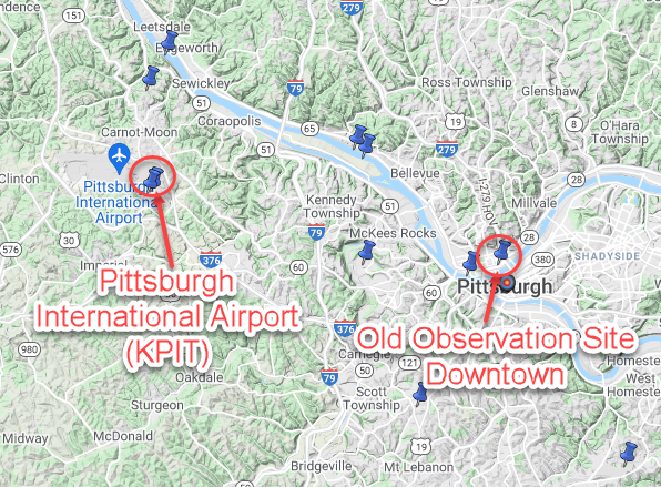
If you're forecasting for the downtown Pittsburgh area (where the city's official observations were taken from 1875 until 1952), its location is about 200 feet lower in elevation and about 10 miles east of Pittsburgh International Airport--KPIT (where the city's official observations have been taken since 1952). Recalling from previous studies that higher elevation locations tend to be a bit cooler than their lower elevation counterparts (all else being equal), it stands to reason that the specific climatology of the two locations might differ, at least slightly.
Since the location of official observations has changed over time in many large cities, scientists at NOAA have created what's called ”ThreadEx“ data (opens in a new window), which is a "threaded" historical record that stitches together observations from multiple historical observation sites into one "continuous" thread. For cities where a ThreadEx data set exists, it's considered the city's official climate record. For Pittsburgh, the period of record goes back to 1875, even though the period of record from KPIT at the airport doesn't go back nearly that far.
ThreadEx data is a great starting point to understand a city's climatology, but using it by itself can be problematic. Are the observations taken at the old observation site in downtown Pittsburgh (200 feet lower in elevation and more in the midst of the urban heat island) representative of conditions at the airport? Not really. For example, if we examine the history of the hottest days on record in Pittsburgh (opens in a new window) (highs of 100 degrees Fahrenheit or higher), it's easy to see that most of them occurred prior to 1952, when the official observation site switched to KPIT. In other words, historically, 100-degree days are more common downtown than they are at KPIT. In fact, two dates exist when the downtown observation site reached 100 degrees Fahrenheit and weather records were also being taken at KPIT. The highs at KPIT on those days were 99 degrees and 96 degrees, providing further evidence that 100 degrees is a harder threshold to reach at the higher elevation of the airport.
Forecast Tip
If you want to really dig into a city's climatology, just using the official climate record (the ThreadEx data) may not be sufficient. If climatological data exists for the exact location where your forecasts are being verified, the data for that site may be more useful, even if its period of record is shorter (as long as it's not too short). More information for retrieving a city's climate data is coming later in this section.
What Exactly is "Normal" Anyway?
When studying a location's climatology, a common place to start is with "normal" temperatures and precipitation. But, what does "normal" really mean? In your previous studies, you learned that normal temperatures are essentially 30-year averages, which get updated once every decade. That's basically true, but there's a little more to it than that. As it turns out, raw averages over a 30-year period can be a bit noisy, where one or two very warm / cold / wet days in the sample can skew the average for that date a bit. So, to eliminate the noise and paint a clearer picture of day-to-day and seasonal trends, the raw averages undergo some statistical smoothing to create the official climate normals for a given city. To see the difference between raw averages and official 1991-2020 normal high temperatures for State College, Pennsylvania, check out the graph below.

The blue line on the graph, which represents the raw average of daily high temperatures from 1991 to 2020 shows a number of "bumps" that are just noise and have no meteorological significance (a few are highlighted on this annotated version of the graph (opens in a new window)). So, to avoid being misled by the noise in day-to-day raw averages, forecasters typically prefer using the official (smoothed) normals (orange line). With precipitation, the "noise problem" with raw averages gets even worse (check out the corresponding graph for daily raw average and official normal precipitation at State College (opens in a new window)). The abrupt spikes and lulls that occur on a day-to-day basis are noise, so official (smoothed) normals are calculated to better identify seasonal trends. Note that there is a slight uptick in daily normal precipitation in the warm season (daily normals are generally greater than 0.10 inches), but it's hard to tell from the raw averages.
Forecast Tip
Official climate normals (which are commonly communicated to the public) are typically more useful for understanding average day-to-day weather behavior at a particular location than 30-year raw averages. Official normals are statistically smoothed values and typically get reported as whole numbers for temperature and as inches of liquid (to the nearest hundredth) for precipitation, which is consistent with measurement practices in both cases in the U.S.
What Records are Important?
While normals tell forecasters the (approximate) 30-year average conditions at a location, it's also helpful to know the extreme (record) values of temperature and precipitation. You may be most accustomed to "record high" and "record low" temperatures since they're what most commonly get reported, but they don't tell the entire story of temperature extremes.
For example, if forecasters wanted to know what constituted an extremely hot day at a particular location during a particular time of year, they would look up the record maximum temperature (or, "record high") for the date (and perhaps some surrounding days, too). But, the record maximum temperature only tells us the historical upper bound for maximum temperatures on a given date. The historical lower bound for maximum temperatures is important, too, because it lets forecasters know what constitutes an extremely cool (or cold) "daytime" in most cases. Knowing the record maximum temperature and recorded lowest maximum temperature for any given date tells the forecaster what the historical range of maximum temperatures is for the date.

Knowing the range of historical maximum temperatures at a given time of year can be of great use to forecasters. For example, the graph above shows record daily maximum (red dots) and daily record lowest maximum temperatures (blue dots) at State College, Pennsylvania for each day during the year. Very quickly, we can see that an extremely hot day during the hottest time of year (mid-July) in State College would have high temperatures in the upper 90s to low 100s. On the flip side, a very cool mid-July day would have high temperatures in the 60s! In mid-winter, the warmest days in January historically have had high temperatures in the 60s mainly, while the coldest days have had high temperatures in the single digits, or (in a few cases) even below zero.
The same idea applies to daily minimum temperatures. The daily record minimum (or "record low") tells forecasters the lower bound for minimum temperature. But, to get a complete picture of daily minimum temperatures, we need the upper bound, too -- the record highest minimum temperature, which tells us what constitutes an extremely mild or warm night (in most cases) at a given time of year. Precipitation, on the other hand, is a bit of a different story. Yes, daily record maximum precipitation values tell us the greatest amount of liquid precipitation that has fallen on any particular day, but the daily record minimum precipitation value would presumably be zero everywhere on Earth (it's pretty safe to assume that it's been totally dry at least once on every calendar day, everywhere).
Key Data Resource
Where can you find daily temperature and precipitation normals and records for a particular city? On the NWS Climate Page (opens in a new window), click on the NWS forecast office on the map that includes your desired location, and then select NOWData to access the data you need. On the list of NOWData stations, note that "[CityName] Area" represents the city's ThreadEx data. If you want data from a specific site (such as a major airport), you'll need to find the specific location on the list. Select, "Daily / Monthly Normals" for normal daily high and low temperatures and precipitation and the official normals will be displayed in several tables beneath a graph. For record temperatures and precipitation, select "Calendar Day Summaries" and the appropriate variables (for example, the variable "Min Temp" and summary type "Daily Maximum" will give you the record highest minimum temperatures for each day).
The bottom line: For maximum temperatures, the relevant extremes that mark the historical upper and lower bounds are record maximum temperatures and record lowest maximum temperatures. For minimum temperatures, the relevant extremes are record minimum temperatures and record highest minimum temperatures.
In the next section, we'll focus on how forecasters can analyze local terrain and historical wind observations to further assess a location's climatology. But, before you move on, check out the Quiz Yourself tool, so that you can test your ability to retrieve basic climatological statistics for a given city. The Explore Further section has some additional links that may be of interest to you, as well.
Quiz Yourself...
Imagine that you are going to be forecasting for Pittsburgh, Pennsylvania, with forecasts verified at Pittsburgh International Airport (KPIT). To retrieve some basic climatological stats, use the NWS Climate Page (opens in a new window), along with the guidance above, to answer the questions in the quiz tool below. Can you answer all five questions correctly? If not, make sure that you're searching for the correct variable and using the correct data set.
Explore Further...
If you want to dig a bit deeper into a particular location's temperature and precipitation climatology, you may be interested in the following links:
- Threaded Station Extremes (opens in a new window): The home of ThreadEx data. You can investigate the official station history for many large U.S. cities., as well as gather a limited set of daily records from each available city's ThreadEx data set.
- xmACIS (opens in a new window): This site contains a complete set of temperature and precipitation records for thousands of U.S. stations. The data is from the Applied Climate Information System (ACIS), which is the same database that runs the NWS Climate Page (linked above), but this site has a larger set of reports and graphs that can be generated (and therefore, is a bit less user friendly). Various interfaces into the ACIS database exist online in addition to xmACIS and the NWS Climate Page (SC-ACIS (opens in a new window) is another option with similar functionality), and if you're want to dissect a location's climatology, these sites have tons of data to explore.
Climatology, Part II: Winds and Terrain
Climatology, Part II: Winds and TerrainPrioritize...
When you've completed this page, you should be able to retrieve monthly summary wind statistics from Local Climatology Data documents, interpret key tendencies from wind roses (most / least common wind directions and directions most / least likely to produce fast winds), and analyze important regional terrain features (elevation changes and bodies of water) that may impact a location's climatology, as well as their impacts based on local wind direction.
Read...
The temperature and precipitation statistics that we covered in the last section are a big piece of a particular location's climatological puzzle, but they don't paint the whole picture. A location's wind climatology also provides important clues about typical / atypical weather, and perhaps more importantly, when coupled with knowledge of the surrounding terrain like bodies of water and elevation changes, can help forecasters understand local influences that winds can have on other weather variables (like temperatures and precipitation).
First off, however, it's important to gauge what constitutes "windy" conditions at your forecast location. Perhaps you've never dug into wind data before, but your experience has probably told you that some locations are typically windier than others. Unfortunately, climatological wind data can be somewhat hard to come by because of a relative lack of properly sited observation stations (many privately owned and home weather observing equipment is not set up to measure wind speed at a standard height of 10 meters). Furthermore, publicly available wind data from ASOS sites is generally limited to hourly observations and some summary statistics for stations at larger airports (anything more typically requires some data mining).
Still, we can get a sense for what constitutes a windy day at select forecast locations by viewing summary statistics compiled by the National Centers for Environmental Information. For larger airports in the U.S., they produce "Local Climatological Data" documents, which contain a wealth of statistics, including mean and record wind speeds (sustained and gusts) for each month. For example, compare the historical wind data at Cold Bay, Alaska (opens in a new window) and Seattle, Washington (opens in a new window). Cold Bay is clearly a windier place, with monthly mean wind speeds that are roughly twice those in Seattle. Furthermore, the monthly record sustained wind speeds in Cold Bay are significantly higher, as are the record gusts (multiple months have had gusts of over 80 miles per hour in Cold Bay). The data for monthly record sustained wind speeds and gusts can be particularly helpful for gauging what constitutes unusually fast winds at a particular location during various times of the year.
Key Data Resource
Local Climatology Data documents from NCDC/NCEI (opens in a new window) contain a wealth of climatological statistics and other useful information. In addition to the monthly summaries of wind data described above, they also contain the exact location (latitude / longitude coordinates) and elevation of major airport stations. They also include a brief, but informative climatology discussion toward the end of the document that can really help forecasters get their local bearings.
A very common visualization for studying a location's wind climatology is a wind rose, which is a plot that displays historical wind direction and speed information. You encountered wind roses during your previous studies, and if you need a refresher on how to interpret them, I recommend this quick discussion on the basics (opens in a new window) (keep in mind, however, that display conventions can vary from website to website). Ultimately, wind roses are a great way to quickly assess from which directions winds most and least commonly blow, and assess which directions are more (or less) prone to particularly speedy winds.
Recurrent patterns in winds may become apparent at a particular location because of regional terrain (winds being channeled through mountains or valleys, for example), persistent mesoscale circulations (like sea breezes or mountain-valley circulations), or persistent storm tracks, and these patterns may change throughout the year. For example, check out the wind roses for Miami, Florida (above) from January and July.
Note that the Miami wind roses for January and July look very different. The most frequent wind direction (marked by the longest spoke) is from the north-northwest in January (blowing from that direction nearly 14 percent of the time). Winds from the east and southeast are also fairly common in January, but not quite as common as north-northwest winds. In July, however, east-southeast winds are the most common (occurring nearly 19 percent of the time), and winds from the north-northwest are much less frequent. It's not even close! In fact, if we sum the percentages of winds from the east, east-southeast, and southeast (the three longest spokes), winds from those directions occur nearly 50 percent of the time combined!
Any ideas why winds from those three directions are so common in July? A big part of it is the regular occurrence of sea breezes as the Florida peninsula warms up during the day and a mesoscale sea-breeze circulation develops, resulting in onshore flow at Miami (opens in a new window). During the summer, this onshore flow ushers in slightly cooler, moist air into south Florida. The reliable sea breeze is a big reason why temperatures have only hit 100 degrees in Miami once since records began in 1895 (per the ThreadEx data). Daily record highs in Miami during the summer are typically in the middle and upper 90s, which is comparable to or even lower than many locations that are much farther north in the U.S. So, wind direction, and the trajectory of the air as it approaches your forecast location are important considerations!
Given the forecasting impacts that air trajectories can have, getting the lay of the land around your forecast site and the surrounding region is critical. Large bodies of water and elevation changes are particularly influential. To get a feel for the lay of the land around your forecast location, it's always a good idea to study a detailed topographic map of the local area, in order to judge the local elevation changes and distance from your forecast site. I'll use Los Angeles International Airport (KLAX) as an example. As you can see from the Google map below, the terrain around Los Angeles is complicated! Many terrain features influence the weather at KLAX!

For starters, the Pacific Ocean is just west of the airport, and the coastline wraps around such that the ocean also lies about 15 miles to the south. Therefore, any time low-level winds blow onshore (having a large westerly or southerly component), they'll bring a substantial maritime influence, which during certain times of year can lead to fog or low cloud development. But, given the substantially higher elevations that are located around the Los Angeles Basin (KLAX sits at an elevation of 97 feet), considerable downsloping occurs when low-level winds blow from the northwest all the way around to the southeast.
Such downsloping brings a warming and drying influence (from compressional warming), with the greatest downsloping occurring on northeast and east-northeast flow since that's where the highest elevations are locally. Indeed, within 30 to 40 miles northeast of KLAX, multiple elevations in excess of 7,000 feet can be found! That's a lot of downsloping! Even downsloping from smaller ranges of hills and mountains (like the Hollywood Hills about 12 miles north of the site, or the Palos Verdes Hills about 12 miles south) is considerable. If air parcels descended the Palos Verdes Hills dry adiabatically (warming at a rate of 5.5 degrees Fahrenheit per 1,000 feet), that's worth almost 8 degrees Fahrenheit of compressional warming between the hills and the airport (assuming a starting elevation of 1,500 feet)! So, it pays to study the terrain surrounding your forecast location even for fairly subtle elevation changes. It's worth considering the impacts for even elevation changes of a few hundred feet or more within several miles.
The farther you go from your forecast site, it takes a more significant topographic feature (body of water or elevation change) to make a significant contribution to a location's climatology. In general, it's wise to assess the terrain within several hundred miles for major bodies of water or elevation changes. And, sometimes, the elevation changes don't take the form of well-defined, obvious hills or mountains. To get an idea of how a forecaster might assess the larger-scale terrain around a forecast location, check out the short video below (4:16), which contains a few examples.
Each forecast location can have its own unique topographic influences that are an integral part of its weather and climate, and it’s important to look at both local factors, which may be within only a few miles or tens of miles, and larger-scale regional factors. In this video, I’ll show some examples of the types of larger-scale regional factors that forecasters need to consider. Some of the factors and their influences are fairly obvious, while others might be more surprising. To start, imagine that you’re forecasting for Omaha, Nebraska. Nebraska is located in the Central Plains of the United States, so it’s easy to think that the terrain in the state is flat, but it’s not.
A closer look at a topographic map of Nebraska shows Omaha over here in extreme eastern Nebraska. The official observation site at the airport sits at an elevation of 982 feet, but elevation steadily increases toward western Nebraska. In fact, the town of Scottsbluff, Nebraska sits at an elevation of nearly 4,000 feet! So, there’s an elevation difference of about 3,000 feet between these two cities across the supposedly flat plains, and there are even some higher elevations to the south of Scottsbluff. The elevation changes are very gradual – the distance between Omaha and Scottsbluff is about 400 miles, but they’re elevation changes are still significant. Any wind with a large westerly component will downslope across Nebraska toward Omaha. Of course, farther to the west, just off the map is the Rocky Mountains, so forecasters have to think about downsloping anytime low-level wind flow has a large westerly component across Nebraska toward Omaha. Downsloping causes warming and drying, so if there’s no cold advection occurring, such wind flow can have a considerable warming influence. Even if cold advection is occurring, downslope warming can counteract some or all of it, depending on the speed of the wind and the strength of the advection.
Now, imagine you’re forecasting for Philadelphia, Pennsylvania. Philadelphia International Airport sits at an elevation of 10 feet above Mean Sea Level. But, there are a number of hills west and northwest of the city, so elevations of 300-500 feet are common even within 20 miles of the airport. Back in Central and Northern Pennsylvania, numerous ridge tops in the Appalachians are between 1,000 and 2,000 feet and we’re still less than 200 miles from the airport. The Poconos are less than 100 miles north of Philadelphia, with some elevations exceeding 2,000 feet. So, winds with a notable northerly or westerly component will downslope toward Philadelphia, bringing a warming and drying influence. Off the map to the east, the Atlantic Ocean sits a little more than 50 miles to the east, and Delaware Bay sits less than 50 miles to the south. So, winds from the south or with notable easterly components will bring a maritime influence, which may moderate temperatures and bring moisture.
Finally, let’s look at Portland, Oregon. The airport lies at a low elevation of 19 feet above mean sea level. About 65 miles to the west is the Pacific Ocean, but in between the ocean and Portland is the coastal range, with numerous elevations between 2,000 and 3,000 feet within 40 miles of Portland. So, winds with large westerly components bring a moderating, maritime influence from the Pacific, but they also downslope considerably between the coastal range and Portland. The drying influence makes the airport one of the drier locations in the area, on average. About 30 miles to the east, we get up into the Cascades, with numerous elevations in excess of 4,000 feet, and Mount Hood in excess of 11,000 feet. So, winds with a significant easterly component will downslope significantly from the Cascades toward Portland, also bringing a warming, drying influence.
As I mentioned, each location can have its own unique topographic influences, so forecasters must take the time to get to know the lay of the land, and think through what impacts changes in elevation and bodies of water have on local weather and climate.
From the video, take note that quantitatively estimating elevation changes and the distance of a particular feature from your forecast location is important, as it gives context for how significant a particular feature may be. Performing these types of analyses also helps forecasters understand the influences that various wind directions may have on the weather at their forecast location in terms upsloping (which brings cooling and potential cloud / precipitation development) or downsloping (warming and drying), or a potential maritime influence.
Ultimately, each location can have its own unique topographic influences that are an integral part of its weather and climate, and it's up to the forecaster to analyze the location's surroundings and determine the relevant features and impacts. I hope the sampling of examples gives you an idea of the types of features and influences that forecasters need to look for, and with your fundamental knowledge from your previous studies, you should be able to perform basic analyses like these on your own. If you want a little practice in making these kinds of assessments for yourself, check out the Quiz Yourself section below for a few more examples. In the next section, I'll show you a Case Study detailing how a forecaster might compile relevant climatology information for a particular city.
Key Data Resources
- Wind Roses: The Natural Resources Conservation Service (opens in a new window) has a selection of wind roses (opens in a new window) for many larger U.S. airports. The wind roses are broken down by month and each shows a 30-year climatology for a particular month.
- Topographic Maps: Turning the terrain layer on Google Maps (opens in a new window) can be a good way to analyze local terrain around your forecast site. For larger-scale state maps, the topographic maps from Johns Hopkins University (opens in a new window) are a good source, although you may find others you like around the Internet.
Quiz Yourself...
Question #1
Imagine that you are forecasting for KMAF in Midland, Texas (elevation 2,862 feet). Given these local-scale (opens in a new window) and state-level (opens in a new window) terrain maps (here's the elevation key (opens in a new window)), describe the important topographical features (including reference elevations and distances) and the impacts of wind direction on local weather based on the terrain. Feel free to explore the area around Midland International Air and Space Port in Google Maps (opens in a new window), if you wish.
Answer: Midland is located about 500 miles northwest of the Gulf of Mexico on the Plains of Texas. Elevations near the city don't change very much, but there is a gradual decrease in elevation toward the northeast, east, and southeast, such that elevations fall below 2,000 feet less than 100 miles from the site and continue decreasing from there. Toward the southwest, west, and northwest, elevations gradually increase toward the mountains of West Texas and New Mexico, where elevations exceed 5,000 feet less than 200 miles from the site.
Flow from the southeast would import moisture from the Gulf of Mexico, which combined with gradual upsloping (a cooling mechanism) can sometimes lead to low clouds, fog, and/or drizzle. Some upsloping occurs on any wind with a substantial easterly component. Flow with a large westerly component downslopes from higher terrain in Mexico, West Texas, and New Mexico, which favors compressional warming and drying.
Note that the exact elevation references and distances that you chose may differ from the ones mentioned here, but a good description needed to reference the Gulf of Mexico and the elevation changes to the east and west (along with upsloping and downsloping impacts).
Question #2
Imagine that you are forecasting for KALB in Albany, New York (elevation 280 feet). Given these local-scale (opens in a new window) and state-level (opens in a new window) terrain maps (here's the elevation key (opens in a new window)), describe the important topographical features (including reference elevations and distances) and the impacts of wind direction on local weather based on the terrain. Feel free to explore the area around Albany International Airport in Google Maps (opens in a new window), if you wish.
Answer: KALB is located in the Hudson River Valley, with rolling hills generally ranging from 200-500 feet near the station (lower elevations are near the river, about 6 miles east). The Helderberg escarpment rises to about 1800 feet 11 miles to the west, while about 12 miles to the east, terrain rises up near 2000 feet. Even higher elevations (3000-4000 ft+) lie about 40+ miles northwest and northeast of the site in the Adirondacks and Green Mountains, respectively. The Atlantic Ocean lies about 120 miles south and east of KALB, while Lake Ontario is about 100 miles northwest.
Winds from most directions downslope into Albany, which has a warming and drying influence, with the greatest downsloping occurring on northwest, southwest, and east/east-northeast winds,. This largely inhibits lake-effect precip (and to a lesser extent, clouds) on northwesterly flow. Long-duration southerly – easterly flow brings maritime, moderating influences from the Atlantic, but they are mitigated somewhat (primarily on easterly flow) by downsloping.
A good description needed to reference Albany's valley location, rolling hills nearby, and the higher elevations surrounding it (along with distance and elevation references), as well as the major bodies of water in the region (Atlantic Ocean and Lake Ontario) and potential downsloping and maritime influences.
Question #3
Imagine that you are forecasting for KRDU in the Raleigh-Durham Metropolitan Area in North Carolina (elevation 416 feet). Given these local-scale (opens in a new window) and state-level (opens in a new window) terrain maps (here's the elevation key (opens in a new window)), describe the important topographical features and the impacts of wind direction on local weather based on the terrain. Feel free to explore the area around Raleigh-Durham International Airport in Google Maps (opens in a new window), if you wish.
Answer: Terrain in the Raleigh-Durham metro area is generally rolling with elevations within 100-200 feet of the station elevation of KRDU. Higher elevations start about 10-20 miles west of the area on the Piedmont Plateau (generally 500-1000 feet). Higher elevations in the Appalachian Mountains are located about 150 miles to the west, up to 3000-6000 ft+. The Atlantic Ocean lies about 150 miles east and south of Raleigh, with lower elevations on the coastal plain in the eastern part of North Carolina.
Northwest to west-southwest winds will downslope from the Appalachians and Piedmont Plateau toward KRDU (a warming, drying influence). Winds from the south and those with a large easterly component will have a maritime influence from the Atlantic, with slight upsloping (a slight cooling influence, which combined with moisture from the Atlantic could lead to low cloudiness and precipitation depending on the large-scale weather situation).
A good description needed to reference rolling hills near KRDU, and the higher elevations to the west (along with distance and elevation references), as well as the Atlantic Ocean and resulting downsloping, upsloping, and maritime influences on specific wind directions.
Case Study: A Climatology Example
Case Study: A Climatology ExamplePrioritize...
When you've completed this page, you should be able to create a climatology similar to the one below.
Case Study...
I recommend that you use the example climatology below as a reference guide. It serves as a template that you can follow when you collect climatological information for forecast cities this semester. The most important parts of the example are the annotations (gray text), which provide additional explanations and descriptions about how each piece of data was collected (much of which came from the Local Climatological Data Document (LCD) for Los Angeles International Airport (KLAX) (opens in a new window), a KLAX wind rose, and the NWS Climate Page for Los Angeles (opens in a new window)).
Climatology of Los Angeles International Airport (KLAX)
Time Period
This climatology focuses on February 9-12 and 16-19 (These were the forecast dates for Los Angeles in the WxChallenge forecasting competition in 2021. General time periods are listed on the WxChallenge schedule page (opens in a new window).)
Topography and Geography
Local Time Zone (Conversion from UTC): Pacific Standard Time (UTC-8) (note that if daylight saving time was in effect, the conversion would be to Pacific Daylight Time (UTC-7)).
Station Elevation: 97 feet (Taken from page 2 of the LCD for KLAX (see the annotation for station elevation in the LCD (opens in a new window)).
Station Location: KLAX is located about 10 miles southwest of downtown Los Angeles, just inland from the Pacific Coast, as shown on this Google map (opens in a new window). (Make sure to describe the location of the station with respect to the center of the nearest major city, which can help to assess urban heat island effects).
Important Topographical Features: The Pacific Ocean is located just west and about 15 miles south of KLAX. The southern California coastal ranges line the inland side of the coastal plain that surrounds the airport. About 12 miles south of the airport, the Palos Verdes Hills rise to about 1,500 feet, while the Hollywood and Santa Monica Hills rise to near 2,000 feet about 12 miles north of the station. Other various hills rise to several hundred feet between the airport and downtown LA. A bit farther away, elevations rise in excess of 3,000 feet about 40 miles to the east-southeast and up to 6000-7000 feet + in Angeles National Forest, about 20 miles north and northeast. These high elevations extend off to the northwest, as well. (Generally, bodies of water and regional elevation differences are the important features to note. Make sure to include some reference distances from the station for significant bodies of water, mountain ranges, and even hills (along with representative elevations).

Winds
Wind Rose: The February wind rose is below. (Note that the color-coded key to quantify wind speeds at the bottom of the wind rose can be a bit difficult to read, so here is a zoomed-in version (opens in a new window). Winds on these particular wind roses are expressed in meters per second.)

Frequency (percentage) of the single most common wind direction: Winds from the west-southwest occur roughly 16.5 percent of the time during February (estimate based on the length of the longest spoke).
Directions that are most and least common: Clearly, winds from the WSW, W, and E are the most common (largest spokes). Winds from the SSW, S, SSE, and WNW-NNW are the least common (smallest spokes).
Direction(s) most likely to produce the fastest winds: W, WSW (largest area of green (and some cyan) shading).
Direction(s) least likely to produce the fastest winds: NE, ENE, SSW. Winds from these directions almost never blow faster than 16.5 knots (smallest blue shading along the spokes and minimal, if any, green areas).
Impacts of wind direction on local weather: Onshore wind directions (large westerly components or southerly components) will bring moist, moderating flow, that can lead to fog or low cloud development. Considerable downsloping occurs on winds from the northwest all the way around clockwise to the southeast, as air flows down surrounding hills and mountains into the LA basin. Such flow would have a warming, drying contribution. The most substantial downsloping comes on northeast and east-northeast flow. (Make sure to note the implications of the wind interacting with the topographic features you mentioned earlier in the climatology. Impacts on precipitation and temperature caused by wind flow interacting with bodies of water or elevation changes are particularly important.)
Maximum observed two-minute wind speed for the month (or months): 38 mph = 33 knots (converted from mph to knots from the "Normals, Means, and Extremes" table on page 3 of the LCD—see the annotation for monthly maximum wind speed (opens in a new window)). (Make sure that you don't use the table containing data only from the most recent year).
Temperatures
All data taken from the NWS local climate page for Los Angeles by clicking on "NOWData." I chose data for "Los Angeles Intl, CA" so that I could get data specifically for KLAX (I did not choose the "LA Airport Area" or "LA Downtown Area" options since those are the ThreadEx datasets that may incorporate multiple sites). For normals, I selected "Daily / Monthly Normals" and "Daily" for data type, then retrieved the relevant values from the tables (not the graph). For records, I used "Calendar Day Summaries" and selected my variables accordingly. For daily records, make sure you're using the entire period of record at the station (you may need to enter "por" into the year range if it's not there by default).
Each WxChallenge city consists of two forecasting weeks (4 days each) and forecasts are submitted Monday - Thursday, so the days we're actually forecasting for are Tuesday - Friday. In this section, you want to list the data for each day we're forecasting for (Tuesday - Friday each week). This climatology was prepared in February, 2021 and our forecast days were February 9-12 and 16-19, so the data below come from those dates.
| Date | Normal Maximum (ºF) | Normal Minimum (ºF) | Record Maximum (ºF) | Record Minimum (ºF) | Record Lowest Maximum (ºF) | Record Highest Minimum (ºF) |
|---|---|---|---|---|---|---|
| Tuesday 2/9 | 66 | 50 | 88 | 38 | 51 | 60 |
| Wednesday 2/10 | 66 | 50 | 85 | 37 | 49 | 60 |
| Thursday 2/11 | 66 | 50 | 88 | 36 | 55 | 58 |
| Friday 2/12 | 66 | 50 | 88 | 34 | 53 | 61 |
| Tuesday 2/16 | 66 | 50 | 88 | 36 | 57 | 59 |
| Wednesday 2/17 | 66 | 50 | 87 | 37 | 54 | 58 |
| Thursday 2/18 | 65 | 50 | 82 | 39 | 54 | 60 |
| Friday 2/19 | 65 | 50 | 87 | 38 | 54 | 58 |
| RANGE | 65-66 | All days are 50 | 82-88 | 34-39 | 49-57 | 58-61 |
Precipitation
All data taken from the NWS local climate page for Los Angeles. Data can be retrieved by similar methods used to retrieve daily temperature data.
| Date | Normal (inches of liquid) | Record Maximum (inches of liquid) |
|---|---|---|
| Tuesday 2/9 | 0.10 | 1.66 |
| Wednesday 2/10 | 0.11 | 2.50 |
| Thursday 2/11 | 0.10 | 1.98 |
| Friday 2/12 | 0.11 | 2.15 |
| Tuesday 2/16 | 0.12 | 1.82 |
| Wednesday 2/17 | 0.12 | 1.88 |
| Thursday 2/18 | 0.11 | 1.29 |
| Friday 2/19 | 0.12 | 3.49 |
| RANGE | 0.10-0.12 | 1.29-3.49 |
With a complete climatology at your disposal, you should keep these statistics in the back of your mind (refer to your climatology as often as needed) as you make your daily forecasts. In addition to helping you get to "know" your forecast location and common weather influences, this data will help you see when weather patterns depart dramatically from "normal" and near the extremes. During these times, you'll want to employ some strategies that we'll learn about later in the course.