Lesson 1 Images
Lesson 1. Forecasting Fundamentals
18Z Radar Image

18Z Radar Image.
The image is a weather map displaying part of the Midwest United States, illustrating a derecho. The map is marked with state boundaries. A cluster of green, yellow, and red colors signifies precipitation intensity, with red indicating the heaviest rain. The storm appears concentrated over Iowa and extends into Illinois and surrounding states. Yellow rectangular outlines indicate Severe Thunderstorm Watches. The top-left corner includes a legend showing color codes for rain, mixed precipitation, and snow with a timestamp and source information.
SPC filtered storm reports

SPC filtered storm reports.
The image is a map of the central United States, highlighting storm reports across various states including Nebraska, Iowa, Missouri, Kansas, Illinois, Indiana, and parts of neighboring states. The map displays a network of roads and city names in a subdued color palette. Weather events are marked with symbols: blue "W" for wind, green "H" for hail, and red "T" for tornado. The majority of the symbols on the map are blue "W" symbols, indicating wind reports distributed densely across the Midwest, particularly in Illinois and Indiana. Green "H" symbols are scattered, mainly in Kansas and Missouri. Red "T" symbols, indicating tornado reports, are sparse and appear close to city names like Fort Wayne and Rockford. The map also includes a text box in the lower left corner labeled "SPC 200810 Filtered Storm Reports" with further details.
Assessing Forecast Accuracy
Extended forecasts for blizzards

Extended forecasts for blizzards.
Days of the week are listed as columns on a green background, each with weather conditions depicted for Tuesday through Sunday. Tuesday features a sun partially obscured by a cloud with text "few clouds". Wednesday and Thursday are similar, with "few clouds", depicted by a sun and a cloud. Friday's weather shows "partly sunny" with a sun and cloud. Saturday has "cloudy mild" with a grey cloud and numbers "45" and "36" in red and blue, respectively. Sunday warns of a snowstorm with a snowflake graphic, text "snow 30-35” windy", and temperatures "28" and "15" in red and blue. A cartoon character in a suit and red tie is on the left, smiling with a speech bubble saying, "Better stock-up now, folks. The storm of the millennium is coming."
A Wise Forecasting Philosophy
GFS forecast from the day before the event

GFS forecast from the day before the event.
The image is divided into six panels, each displaying a different type of weather map from meteorological data. The top left panel features a map with red and purple regions surrounded by contour lines. The top middle panel displays a map with tightly packed red and black contour lines and a few red "L" symbols, denoting low-pressure systems. The top right panel shows a map with areas colored in blue, green, and orange, indicating precipitation levels across the northeastern United States over a 3-hour period.
The bottom left panel has green, white, and orange areas representing various relative humidity values with contour lines representing 700-mb geopotential heights. The bottom middle panel includes a map with green and orange areas representing various relative humidity values at 850 mb and darker lines, displaying 850-mb geopotential heights. The bottom right panel is similar to the top right one, showing precipitation levels in blue, green, orange, and red over the northeastern United States, except this panel shows total precipitation over the entire model run.
Deep Moisture Convergence

Deep Moisture Convergence.
The image is a map of the continental United States featuring contour lines indicating deep layer moisture flux convergence. The map is outlined with state borders in brown. Along the eastern U.S. coast, and extending into the Atlantic Ocean, a series of red contour lines are shown. These lines are more densely packed and curve prominently near the coast, indicating higher values or changes in the parameter measured. There are cyan contour lines with numbers, primarily over the Gulf Coast, southern Texas, and the Pacific Northwest, indicating negative values.
It All Starts With Observations
Cotton Region Shelters

Cotton Region Shelter.
The image depicts a Cotton Region Shelter, which is a weather station enclosure, situated outdoors on a metal frame with four legs. The enclosure has a rectangular shape with louvered panels on all sides, which allow for air ventilation while protecting the instruments inside from direct sunlight and precipitation. The screen is elevated on a metal stand with diagonal cross-bracing for stability. The enclosure stands in a gravel area with some small patches of grass and yellow flowers around the base.
Interior of the Cotton Region Shelter

Interior of the CRS.
The image depicts the interior of a Cotton Region Shelter, a white, wooden louvered enclosure used to house meteorological instruments. Inside, there are two thermometers mounted on a horizontal white board. The louvered panels surround the thermometers, allowing air circulation while protecting them from direct sunlight and precipitation. A printed instruction sheet is visible on the right side, attached to the same surface as the thermometers.
Constriction in the bore

Constriction in the bore.
The image shows the tip of a glass thermometer on a neutral background. The thermometer's end is bulbous and contains a shiny, reflective metallic substance, likely mercury. The glass tube is transparent, allowing a clear view of the silver-colored liquid inside.
Barbell-shaped marker

Barbell-shaped marker.
The image shows a close-up view of a thermometer with a glass tube encased in a metal frame. The thermometer contains a red liquid indicating the temperature level. Within the red liquid is a barbell-shaped marker used to help register minimum temperature. The liquid is situated within a narrower section of the glass tube. The upper part of the thermometer features a series of small, evenly spaced black markings and numbers that allow for temperature readings. The metal frame surrounding the glass has a smooth, slightly curved surface and displays some signs of wear, such as minor scratches and discoloration. The image is focused on the central portion of the thermometer, highlighting the red liquid and the graduations.
Maximum Minimum Temperature System

Maximum Minimum Temperature System.
The image shows a meteorological instrument shield mounted on a metal pole, which is attached to a chain-link fence. The shield is composed of several horizontal, flat, circular plates stacked with gaps in between, creating a layered appearance. These plates are off-white and are designed to protect the instrument from environmental elements while allowing air circulation. The background features a grassy field with scattered trees and a distant building, indicating an outdoor setting on a sunny day.
Hygrothermometer

Hygrothermometer.
The image depicts a hygrothermometer mounted on a pole, set against a cloudy sky. The device consists of a cylindrical structure with a rounded dome on top and a flat disc at the bottom. There are several cables connected to the instrument. Adjacent to the cylindrical structure is a metal frame supporting a rectangular box. In the background, dense trees are visible along the horizon under a mostly cloudy sky.
Ultrasonic anemometer

Ultrasonic anemometer.
The image shows an ultrasonic anemometer mounted against a plain, light-colored background. The device consists of a cylindrical body with a white exterior, topped with a dark-colored cap. Three metallic arms extend outward from the top, each angled upward and tipped with a small cylindrical sensor. A thin, pointed rod protrudes upward from the center of the device.
Clear, plastic inner cylinder

Clear, plastic inner cylinder.
The image shows a top-down view of a metallic collection cylinder placed on a surface of gray stone tiles. The cylinder has a smooth, reflective interior surface with a smaller inner cylinder extending upwards from the base. The main cylinder is shiny and appears to be made of stainless steel, while the inner cylinder is consistent in color and texture. In the top right corner of the image, there is an inset photo displaying a different cylinder with a yellowish interior, also placed on a similar tiled surface.
Weighing gauge

Weighing gauge.
The image depicts a weighing precipitation gauge shielded by an array of vertical red and white striped slats. The surrounding slats are arranged in a circular pattern and are mounted on red poles that extend vertically to connect to the top of the structure. The area around the setup is covered with gravel and sparse vegetation. In the background, a chain-link fence and a partly cloudy blue sky are visible.
Tipping-bucket rain gauge

Tipping-bucket rain gauge.
The image showcases a weather station, with a white louvered Stevenson screen mounted on a metal stand. The structure is supported by crisscrossed metal legs and situated on a gravel-covered area. To the right of the Stevenson screen is a cylindrical metal tipping-bucket rain guage, labeled with a danger sign, indicating an electrical hazard. The container is elevated on thin metal legs. In the background, there is a wire fence bordering a pathway, leading to a brick building with large windows.
Close-up view of the top of a tipping-bucket

Close-up view of the top of a tipping-bucket.
The image features a top-down view of a circular, metallic apparatus with an open lid, revealing its internal components. Inside, there is a central vertical rod supporting a horizontal, curved metallic piece that looks aged and slightly rusted. Attached to it is a small setup involving wires and connectors. The inside walls of the apparatus are smooth and painted white, creating a contrast against the dull, metallic tones of the inner components. The outer structure is sturdy, designed with brackets that hold the inner parts in place. It is positioned outdoors, as indicated by the surrounding gravel path.
Fischer Porter automatic rain gauge

Fischer Porter automatic rain gauge.
The image shows a Fischer Porter automatic rain gauge situated outdoors on a patch of grass. The device has a conical top section sitting above a cylindrical base, both painted light gray. The rain gauge is mounted on a small rectangular platform that appears to be made of wood or concrete. A solar panel is attached to a metal post next to the device, which is affixed to the platform.
Punched ticker tape

Punched ticker tape.
The image shows a close-up of a mechanical device that processes ticker tape, housed within a metal enclosure. The central element is a strip of punched ticker tape running vertically through the machine. The tape has numerous small holes arranged in patterns along its length. On the right side, there is a circular dial with multiple markings and a central knob. Adjacent to it is an arrow that seems to indicate measurements or positions on the dial. The device also features a box-like component with visible knobs and buttons; a handwritten label is attached to this component. The interior of the enclosure is metallic and somewhat industrial in appearance, with various connectors and wiring visible.
Climatology, Part I: Temperature and Precipitation Stats
History of the Hottest Days on Record in Pittsburgh

History of the Hottest Days on Record in Pittsburgh.
The image is a bar graph showing the number of days with maximum temperatures of 100°F or higher from January through December in the Pittsburgh area, Pennsylvania. The graph spans from 1875 to 2021 and is divided into two sections by a dashed red vertical line. The left section, titled “Official Observations Recorded Downtown,” covers the period from 1875 to 1951, while the right section, titled “Official Observations at KPIT (Airport),” covers 1952 to 2021. The y-axis represents the "Number of Days" ranging from 0 to 6. The x-axis represents the years.
Blue bars indicate the occurrence of such high-temperature days, with notable peaks around the late 1870s and 1880s in the downtown section, and additional peaks in the years 1916, 1934, 1941, 1988, and 1995 in the airport section.
Annotated Version of the Daily Normal vs. Raw Average High Temperature Graph

Annotated version of the daily normal vs. raw average high temperature graph.
The image is a line graph depicting daily normal and raw average high temperatures for State College, Pennsylvania, across a year. The x-axis represents dates from January 1st to December 31st, while the y-axis shows temperature in degrees Fahrenheit, ranging from 0 to 90. Two lines are charted: a blue line for the "1991-2020 Raw Average" and an orange line for the "1991-2020 Official Normal," which run parallel closely, except for differences such as those highlighted by three red ovals. These ovals indicate periods where the raw average deviates from the official normal significantly. The graph peaks around July, with temperatures just above 80°F, and is lowest in January and December, around 34°F.
Corresponding graph for daily raw average and official normal precipitation at State College

Corresponding graph for daily raw average and official normal precipitation at State College.
The image is a line graph titled "State College, Pennsylvania Daily Normal and Raw Average Precipitation." It shows two data trends over a year, comparing precipitation levels. The x-axis represents dates from January 1 to December 31, spaced every week or so. The y-axis indicates precipitation in inches, ranging from 0 to 0.5. An orange line illustrates the 1991-2020 raw average precipitation, showing significant fluctuations throughout the year with peaks during various months. A gray line demonstrates the 1991-2020 official normal precipitation, which is relatively stable compared to the raw average. The legend at the bottom identifies the orange line as "1991-2020 Raw Average" and the gray line as "1991-2020 Official Normal."
Climatology, Part II: Winds and Terrain
Wind data at Cold Bay, Alaska

Wind data at Cold Bay, Alaska.
The image is a detailed table titled "Normals, Means, and Extremes" for Cold Bay (PACD). It provides climatological data across various categories such as temperature, heating and cooling degree days (HDD and CDD), relative humidity (RH), percent possible sunshine, thunderstorms, cloudiness, pressure (PR), winds, and precipitation. The table spans monthly statistics from January to December, including yearly totals or averages, and is organized into rows and columns. Key focus areas of the table are highlighted in red, particularly related to wind data such as mean speed, maximum and record speeds, and their occurrences. The table is dense with numerical data, with shaded sections for annotations.
Wind data at Seattle, Washington
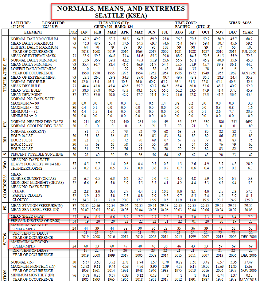
Wind data at Seattle, Washington.
The image is a detailed data table titled "Normals, Means, and Extremes Seattle (KSEA)" showing various meteorological statistics for Seattle. It covers different elements such as temperature, heating and cooling degree days, relative humidity, cloudiness, pressure, winds, and precipitation. The table spans twelve months from January to December, as well as a yearly average, with columns dedicated to each. Key sections are highlighted, particularly the wind speed and direction statistics. The highlighted area displays data for mean wind speed, prevailing wind direction and speed, maximum wind speeds, and directions for specific occurrences, along with their year of occurrence. The table includes the observational period for each element, referenced as "POR."
Onshore flow at Miami

Onshore flow at Miami.
The image is a satellite view map of southern Florida, showing a detailed layout of the region's geography and urban areas. It focuses on the eastern coastline where cities like Miami, Hollywood, and Fort Lauderdale are highlighted. The map extends to the Bahamas to the east, shown with distinct turquoise waters differentiating the ocean and islands. Miami International Airport is marked with a red pin, and yellow arrows point from offshore into Miami. Main highways and roads are visible, along with natural features like the Everglades National Park to the southwest and Big Cypress National Preserve to the west. The Gulf of Mexico lies on the western coast of Florida, and the Atlantic Ocean is to the east.
Los Angeles International Airport area (Full-sized image)

Los Angeles International Airport area (Full-sized image).
The image is a map of the Los Angeles area and its surrounding regions, highlighting various geographic features with green shaded relief to indicate parks or forest areas. The map includes major cities, highways, and natural landscapes. Key features are marked with red arrows pointing to specific locations:
- The "Hollywood / Santa Monica Hills" approximately 2,000 feet, located near Santa Monica and Malibu.
- The "Palos Verdes Hills" around 1,500 feet, south of Torrance.
- The "Angeles National Forest," about 7,000 feet and above, located northeast of Los Angeles.
- The "Santa Ana Mountains," above 3,000 feet, situated southeast of Los Angeles.
The Los Angeles International Airport is marked with a red pin, indicating it as a significant landmark. Major cities like Los Angeles, Glendale, Pasadena, and Santa Clarita are shown, along with major highways such as I-5, I-405, and US-101.
KMAF Local-scale Terrain Map

KMAF Local-scale terrain map.
The image is a map focusing on the area around Midland and Odessa in Texas. The map highlights major roads, cities, and geographic divisions. Midland is prominently marked in the center with a red pin labeled "Midland International Air & Space Port," indicating a point of interest. Surrounding cities, such as Odessa, Gardendale, Andrews, and Big Spring, are marked and connected by highways. The map uses a light color palette with beige representing land and blue for water bodies. Green patches indicate parks or green spaces.
KMAF State-level Terrain Map

KMAF State-level terrain map.
The image is a topographic map illustrating the state of Texas with an emphasis on elevation through a color gradient. It uses diverse colors to indicate variations in elevation, with reds and purples for higher elevations in the western region transitioning to greens and blues for the lower elevations in the east. A red outline marks Texas's state boundaries, and various cities are highlighted with white dots and labels. Specific cities include El Paso, Amarillo, and Houston among others. Geographic features such as plains and plateaus are subtly indicated through shading and color variations.
Elevation key
Elevation key.
The image shows a vertically oriented, color-coded elevation key, with elevations ranging from 0 feet at the bottom up to more than 13,000 feet at the top. Colors gradually transition as elevations increase.
KALB Local-scale
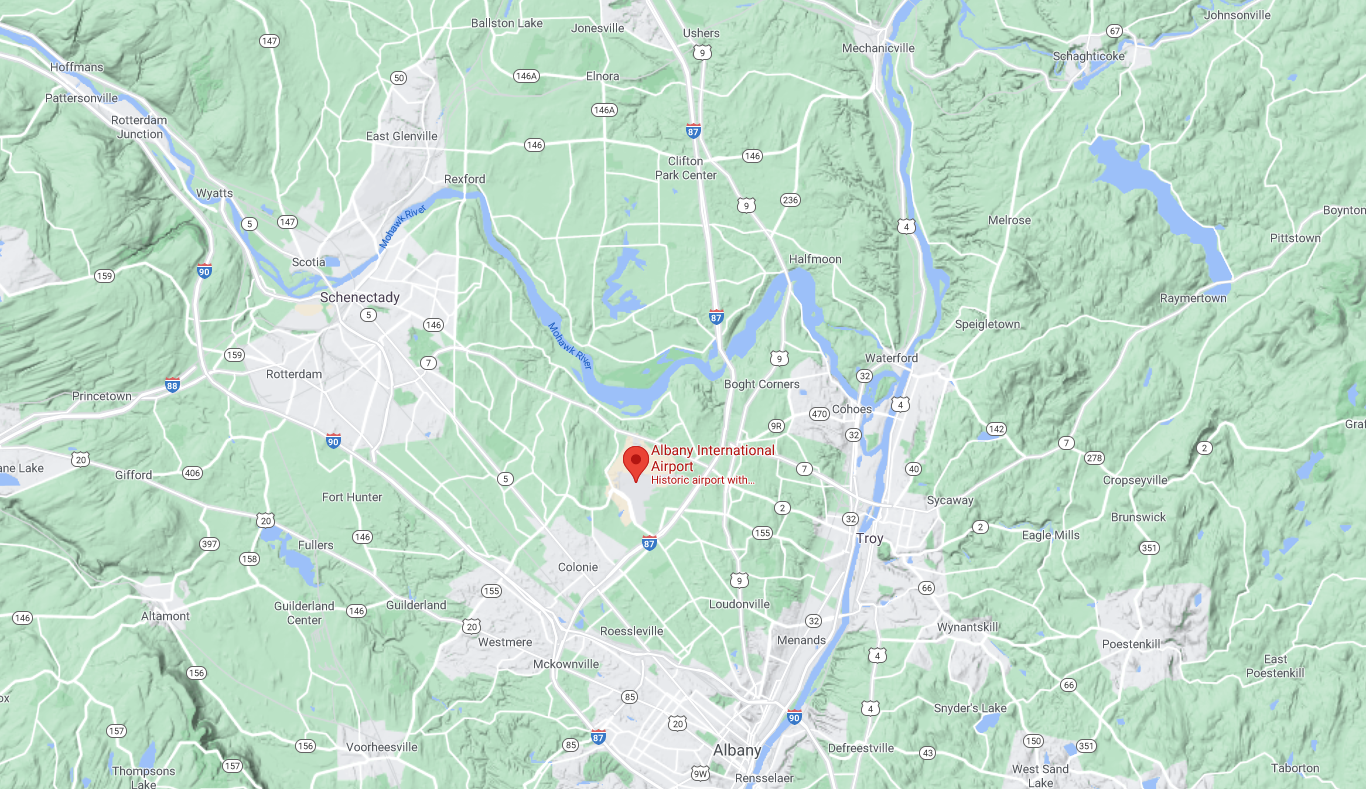
KALB Local-scale.
The image is a detailed map of an area around Albany, New York. It shows a network of roads and highways, green areas representing forests or parks, and bodies of water such as rivers and lakes. Prominent cities and towns, including Albany, Schenectady, and Troy, are labeled. Various routes like the Interstate 87 (I-87), Interstate 90 (I-90), and smaller roads are visible. The central feature is a red pin marking "Albany International Airport," located in a region with mixed urban and rural geography.
KALB State-level

KALB State-level.
The image is a colored topographic map depicting the northeastern United States, focusing on New York State and its surrounding areas. The landscape features a mix of various elevations represented in different colors; higher elevations are shown in brown and lower areas in green. Bodies of water are depicted in blue. The map displays major cities and locations marked with white dots and labeled in white text. A red line outlines a specific geographical boundary. The map includes major cities and landmarks such as Buffalo, Rochester, Syracuse, Albany, and New York City. Latitude and longitude are indicated along the left and bottom edges, respectively.
KRDU Local-scale

KRDU Local-scale.
The image shows a map of the Raleigh-Durham region in North Carolina, highlighting the Raleigh-Durham International Airport with a red pin. The map depicts a mix of urban areas, primarily marked in light gray, and large expanses of green, indicating forested or rural areas. Major highways and roads are visible as white lines crossing the map. Several cities and towns are labeled, including Durham, Chapel Hill, Cary, and Raleigh. Water bodies such as Jordan Lake are shown in blue. The map is oriented with north at the top.
KRDU State-level

KRDU State-level
The image is a colorful topographic map of North Carolina, showing elevation and major cities. The western part features the Appalachian Mountains, depicted in shades of red and purple, indicating higher elevation. The central and eastern regions transition into green and blue tones, showing flatter, lower land. Various cities are marked with white dots and labeled in white text, including Asheville, Charlotte, Greensboro, Raleigh Durham, Fayetteville, and Wilmington. The map includes latitude and longitude lines and spans from approximately 76 to 84 degrees in longitude and 33.5 to 36.5 degrees in latitude. The state boundary is outlined in red, and the Atlantic coastline is visible on the eastern edge.
Case Study: A Climatology Example
Annotation for station elevation in the LCD

Annotation for station elevation in the LCD.
The image is a table displaying meteorological data for Los Angeles (KLAX) for the year 2020. It provides detailed temperature information for each month, including mean daily maximum and minimum, highest and lowest daily temperatures, and the occurrence dates for these extremes. Additional parameters such as average dry bulb temperature, mean wet bulb, and mean dew point are listed. The table also indicates the number of days with temperatures meeting specific criteria, alongside heating and cooling degree days. The top presents geographical and elevation information with latitude at 33° 56'N and longitude at 118° 23'W. Ground elevation is 97 feet. The time zone is noted as Pacific (UTC -8), and the WBAN number is 23174.
KLAX Google map

KLAX Google map.
The image is a detailed map of the Los Angeles area, highlighting major roads, cities, and natural features. The area in the map is predominantly urban and spans from the Pacific Ocean on the left to inland cities on the right. Prominent city names include Los Angeles, Santa Monica, Long Beach, Anaheim, and Pasadena. Major highways such as I-405, I-10, and I-5 are indicated with blue shields. Green areas signify parks and mountain ranges, including Topanga State Park and Chino Hills State Park. The ocean appears as a large blue expanse on the left side of the map. A red location marker labels "Los Angeles International Airport" along the coast near Manhattan Beach.
Wind rose zoomed-in version

Wind rose zoomed-in version.
The image is a data table with text regarding wind speed. On the left side, there is a color legend indicating different wind speed ranges in meters per second (m/s). The colors range from cyan for speeds greater than 11.05 m/s to black for speeds between 0.51 and 1.80 m/s. The table on the right is divided into several sections containing details such as the modeler name, date, company name, wind speed display, average wind speed, calm winds percentage, wind orientation, and plot year-date-time information. The cells in the table contain specific numerical data and textual information.
Annotation for monthly maximum wind speed

Annotation for monthly maximum wind speed.
The image is a detailed climate report titled "Normals, Means, and Extremes: Los Angeles (KLAX)." It presents various climate elements such as temperature, heating and cooling degree days, percentage possible sunshine, cloudiness, pressure, and wind data for Los Angeles. The data is organized in a tabular format with rows and columns, covering each month of the year along with annual summaries. Specific metrics include normal daily maximum, mean daily maximum, and highest daily maximum temperatures, among others. Detailed measurements such as heating and cooling degree days, percent possible sunshine, and mean sea level pressure are also included. Wind data includes mean speed, prevalent direction, and maximum speeds. The table notes latitude, longitude, elevation, time zone, and WBAN identifier at the top.