Read...

Way back in Lesson 3, we talked about how solar radiation from the Sun strikes the Earth differently in different seasons. For Northern Hemisphere summer, the Earth's north pole tilted toward the Sun and vice versa for the winter. This is why we have longer days in summer than in winter. The geometry of Earth's annual orbit around the Sun changes slowly over time. These changes are subtle, but they are persistent over thousands of years and have a profound impact on climate.

Obliquity

The first of these changes involves the tilt angle (or, more technically, the obliquity) of Earth's axis relative to its orbital plane. Today, the Earth's rotational axis is inclined at an angle roughly 23.5 degrees from the vertical to the orbital plane. This is why the tropics are located between 23.5°N and 23.5°S and why the Arctic and Antarctic circles are poleward 66.5°N and 66.5°S (90°-23.5°=66.5°), respectively. This angle of inclination is not fixed over time, however, and it varies between roughly 22.1 degrees and 24.3 degrees. Seasonality only exists because of the tilt; if not for the tilt, neither hemisphere would be preferentially tilted toward the Sun at any time of the year. Therefore, periods, when the tilt angle is greatest, are periods of heightened seasonality, while periods, when the tilt angle is smallest, have reduced seasonality. It takes roughly 41 thousand years (41,000 years) for the tilt angle to go through one full cycle of alternation between minimum and maximum values of the obliquity.

Video: Changes in Obliquity (Tilt) (:01) (No Audio)

Wobble

The second of these orbital variations involves the slow wobble (or, to use the more technical term, the precession) of the Earth's rotational axis. This is analogous to the wobbling of a gyroscope. One full wobble takes roughly 19-23 thousand years (19,000-23,000 years). The precession determines when the Northern and Southern Hemispheres are each tilted toward (summer) or away (winter) from the Sun.

Video: Axial Precession (Wobble) (:04) (No Audio)

The primary importance of this factor is that it determines whether the summer solstice in each hemisphere occurs when Earth is farthest (making summer a little cooler) or closest (making summer a little warmer) to the Sun. This factor only matters, then, because Earth's annual orbit around the Sun is not circular but slightly elliptical – which brings us to our last factor.

Eccentricity

The last of Earth's changing orbital parameters involves the ellipticity (or, to use the more technical term, the eccentricity) of the orbit. Another way to think about this in non-technical terms is the "ovalness" of Earth's path around the Sun. Earth's orbit is not circular but, instead, is slightly elliptical. The degree of ellipticity is measured by the eccentricity, which ranges from roughly zero (an essentially circular orbit) to a maximum of roughly 4% (a slightly elliptical orbit). It takes roughly 100 thousand years (100,000 years) for the eccentricity to go through one full cycle of alternation between low and high eccentricity.

Video: Changes in Eccentricity (Orbit Shape) (:07) (No Audio)

These orbital cycles were first discovered by a mathematician named Milutin Milankovitch. Recreating past and future values of these orbital parameters is straightforward using celestial mechanics (a branch of astronomy that deals with motions of objects in outer space) and Milankovitch did these calculations by hand back in the early 1900’s.

The most important part of these orbital parameters is that they impact where solar radiation hits the Earth. Based on his calculations, Milankovitch theorized that the amount of solar radiation hitting the Northern Hemisphere could swing by 20% depending on the relative phases of these cycles. This has significant impacts on the climate system. In the next section, we will discuss how these can lead to large swings in the Earth’s temperature during glacial-interglacial periods.

Let's review these three important concepts. Think about what they mean -- if you can't define it in your head, click to expand and make sure "you hammer it home!"

Obliquity (Tilt)

This refers to the angle between Earth's rotational axis and the vertical to its orbital plane around the Sun. Earth's tilt changes slightly over a cycle of about 41,000 years, varying between approximately 22.1° and 24.5°. Changes in obliquity affect the severity of the seasons: a greater tilt means more extreme seasons (hotter summers and colder winters), while a smaller tilt leads to milder seasons.

Precession (Wobble)

Precession is the slow wobble of Earth's rotational axis, similar to the wobbling of a spinning top. This wobble occurs over a cycle of roughly 19,000 to 23,000 years. Precession alters the timing of when each hemisphere is tilted toward or away from the Sun, affecting the timing of the seasons in relation to Earth's position in its orbit.

Eccentricity (Ellipticity)

Eccentricity describes the shape of Earth's orbit around the Sun, which changes from being more circular to more elliptical over a cycle of about 100,000 years. When the orbit is more elliptical, the distance between Earth and the Sun varies more throughout the year, influencing the amount of solar energy Earth receives and impacting long-term climate patterns.

Read...

Glacial-Interglacial Periods

If you had an eagle eye, you might have noticed on the first page of this lesson that the planet's temperature has experienced large regular swings over the past 500,000 years. See the zoomed-in figure below, where the blue and green lines are temperature reconstructions from ice core data in Greenland and northern Russia, respectively. These large swings are called glacial-interglacial cycles.  Looking at the time between each peak in temperature, you will see that these cycles occur roughly every 100,000 years. Why do these oscillations occur?  Why do they have a regular period of 100,000 years?  What explains their “sawtooth-like" shape where the temperature increases rapidly and then decreases slowly? These are all good questions -- let's see if we can answer them!

The previous section of this lesson taught us about three orbital cycles that occur on long timescales (protip: you should pause here and test yourself to see if you can list the three!). The eccentricity of Earth’s orbit, in particular, operates with a period of 100,000 years. This sounds suspiciously like it could be related to the glacial-interglacial cycles! The question is how?

First, let’s think about how these three orbital parameters alter where and when solar radiation hits Earth. In short, we have stronger seasonality when Earth is more tilted, and when precession causes Earth’s Northern Hemisphere to tilt toward the Sun (summer) at a point when it is closer to the Sun. Think about it: when Earth’s axis is tilted more, the poles experience more extreme seasonal differences. If, during this time, Earth is also farther away from the Sun during Northern Hemisphere summer due to precession, summers—while still warmer than winter—become less hot. These impacts are amplified when the eccentricity of the orbit is greater—that is, their role is "turned up" the more oval-shaped Earth's orbit becomes.

When summers are cooler in the Northern Hemisphere due to a combination of these factors, snow and ice are less likely to melt fully. So, what role does ice play in all of this? Excellent question—we need to explore another (very) important feedback in the climate system.

Ice-Albedo Feedback

Let’s dive deeper into the ice-albedo feedback, a process that can amplify the impact of the orbital parameters we’ve just discussed. Remember when we talked about solar radiation earlier in this class? That’s where we first encountered the concept of albedo. To refresh your memory: albedo is a measure of how much sunlight a surface reflects. Snow and ice have a high albedo, meaning they are excellent at reflecting incoming sunlight back into space, which helps keep the surface cool. In contrast, the ocean or land beneath the snow and ice has a much lower albedo, meaning these surfaces absorb more sunlight, which warms the surface.

Now, let’s consider what happens when there’s less ice than usual. In this scenario, more of the low-albedo ocean or land would be exposed, causing more sunlight to be absorbed rather than reflected. More absorption of solar radiation means more "energy in" and a warmer surface. This additional warmth would melt even more snow and ice. As the ice melts, the exposed surface area with low albedo increases, which leads to even more absorption of solar energy. This results in further warming, which melts more ice, and the cycle continues.

This process is an example of what we call a positive feedback. Essentially, an initial change (in this case, less ice) triggers a series of events that reinforce and amplify the original change.

The ice-albedo feedback is a powerful mechanism in the climate system. It’s one of the reasons why relatively small changes in Earth's orbital parameters can lead to such dramatic shifts in global temperatures during glacial and interglacial periods. The more ice melts, the more the Earth warms, and vice versa. This feedback loop plays a key role in amplifying the natural variability introduced by the orbital cycles.

Read...

Ready to add another recipe to your book? Let's write "How to make an ice age."

Let's put the two concepts we just learned together. Roughly every 100,000 years, the eccentricity of Earth's orbit reaches a high value, creating the largest possible differences in Earth-Sun distance over the course of the year. During these times, there's a point in the much faster 19,000-23,000 year precession cycle when Earth is tilted toward the Sun at its closest approach. This makes summers exceptionally warm and winters unusually cold. This effect is further amplified when the obliquity (tilt of Earth's axis) is at its maximum. We focus on the Northern Hemisphere because there's more landmass, allowing snow and ice to form further south. Typically, winter temperatures are cold enough to maintain ice, but very warm summers lead to rapid melting of snow and ice.

In the figure below, we can see the three orbital parameters—precession, obliquity, and eccentricity—plotted over time. Notice how these cycles oscillate at different frequencies: precession is the fastest, followed by obliquity, with eccentricity being the slowest. Also shown in this figure is the summer Northern Hemisphere insolation (solar radiation received at 65°N). If you look very closely, you'll see how this insolation pattern is linked to the orbital cycles: broad changes every 100,000 years from eccentricity, with smaller, faster changes from precession and obliquity. Lastly, the ice core temperature record offers a glimpse into Earth's past climate, where you can clearly see the sawtooth pattern of glacial-interglacial cycles, occurring roughly every 100,000 years.

Let's focus on one glacial-interglacial cycle in particular. First, note that in this graph, time progresses to the left, opposite to what we've usually seen -- there's nothing wrong with this, but you need to flip your brain to think "hey, the present day is on the very left of this plot." Starting at point A, we see a period of very cold temperatures—an ice age—followed by a rapid increase in temperature. This warming coincides with an increase in Northern Hemisphere summer insolation at 65°N, along with a rise in eccentricity and high obliquity and precession values. As described earlier, this combination of factors—greater eccentricity amplifying the effects of precession and obliquity—leads to warmer summers that quickly melt ice, triggering a positive feedback loop that pulls Earth out of the ice age.

At point B, both precession and obliquity are in their negative phases, and eccentricity begins to decrease. This reduces solar radiation at 65°N, leading to warmer winters and cooler summers in the Northern Hemisphere. These conditions are perfect for growing ice sheets: warmer winters allow for more snowfall (since warmer air holds more moisture), and cooler summers prevent accumulated snow from melting. Ice begins to build up, reflecting more solar radiation back to space and causing cooling to spread southward. This is how a glacial period slowly takes hold, lasting tens of thousands of years. The sawtooth pattern of Earth's temperature comes from the fact that melting ice happens faster than its accumulation, leading to quicker warming followed by slower cooling.

Milankovitch cycles graph.

Credit: Milankovitch Cycles is licensed under CC BY-SA 3.0. 2008.

Let’s return to the full reconstruction of Earth’s climate history that we looked at earlier (I’ve copied it below—trust me, you’ve seen it before!). You might notice something interesting: these ice ages didn’t start showing up until about 700,000 years ago (the wobbles beginning in the fourth panel). Why weren't there more ice ages in the earlier panels? The mechanism we discussed for glacial-interglacial cycles relies on the formation of large ice sheets, and scientists think that the climate just wasn’t cool enough yet to allow for that. While we can’t say for certain, the leading theory is that the planet needed to cross a cooling threshold for large ice sheets to form. This gradual cooling is thought to have been driven by a slow decline in carbon dioxide concentrations over millions of years. In other words, during the time of the dinosaurs, for example, the planet was simply too warm for the ice-albedo feedback to kick in. Eventually, as the Earth continued to cool with age, it reached that critical point, allowing the 100,000-year cycles we see in blue below (and in the figures above) to begin.

Reconstructured global temperature anomaly over the past 500 million years.

Credit: Temperature of Planet Earth by Glen Fergus is licensed under CC BY-SA 3.0.

The glacial-interglacial cycles we observe, driven by Earth's orbital changes and amplified by feedback loops like ice-albedo, have only become prominent in the last 700,000 years as the planet's temperature gradually dipped, allowing large ice sheets to form and trigger these dramatic climate shifts. Pretty "cool!"

Read...

As we've learned, the sun is our primary source of energy. While it's incredibly consistent to the point where we actually define the amount of energy coming into the climate system as the solar constant there are tiny fluctuations in the amount of energy it releases. One of the most intriguing features related to these variations is sunspots—dark blotches or patches on the Sun’s surface that have been observed by humans for centuries. In fact, sunspots were regularly reported in Chinese literature as far back as the 4th century. In 1609, Galileo, with his newly invented telescope, was able to observe them in greater detail, documenting their presence by counting the number of visible spots. Now I should note that you should never (ever!) stare directly into the sun! However, before we talk about the science behind sunspots and their impact on the climate, here's a way you can observe the sun if you want to go sunspot hunting right now or maybe after you finish this lesson!

Sunspots

Sunspots are dark patches on the Sun’s surface that appear cooler and emit less solar radiation than the surrounding areas. Though they may last anywhere from a day to several months, they are constantly changing and shifting. Their size can vary dramatically, ranging from about 100 kilometers to a staggering 10,000 kilometers—larger than the Earth! At any given moment, only about 0.0 to 0.1% of the Sun's visible surface from Earth is covered by sunspots. These spots form due to disturbances in the Sun’s magnetic field, disrupting the normal flow of energy.

In the figure below, we have images of the Sun’s surface taken on two different days—April 29, 2002, and April 29, 2009. The visible light images (which represent what we’d see with our own eyes) show a stark difference in the number of sunspots for the two days. On April 29, 2002, you can spot a large number of sunspots as dark spots scattered across the Sun, while on April 29, 2009, no fewer sunspots are apparent. If you look at the ultraviolet images, you’ll also notice something else—bright regions surrounding the sunspots. These are called faculae. The word "faculae" is borrowed from the Latin for "little torch." While sunspots emit about 15% less solar radiation, the faculae around them are actually more intense, releasing 25% more solar radiation. So, even though sunspots themselves are darker and cooler, the existence of these faculae can actually lead to an overall increase in the amount of solar energy reaching Earth when more sunspots are present!

Total Solar Irradiance (TSI)

The existence of sunspots tweak the amount of energy the Earth recieves from the sun -- what does that mean for us? Thanks to the advent of satellite measurements, we can now directly measure the Sun’s energy output—this is known as the total solar irradiance, or TSI for short. Earth-orbiting satellites are equipped with extremely precise instruments capable of detecting even small changes in TSI. However, these measurements aren’t always perfectly accurate, and the average values of TSI can vary between satellites. To address this, scientists adjust the data, stitching together measurements from multiple satellites to create a continuous and reliable record.

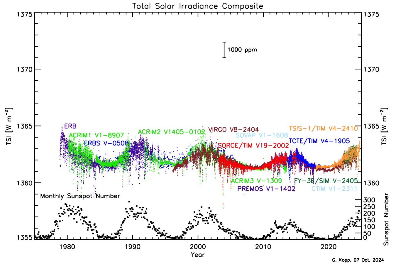
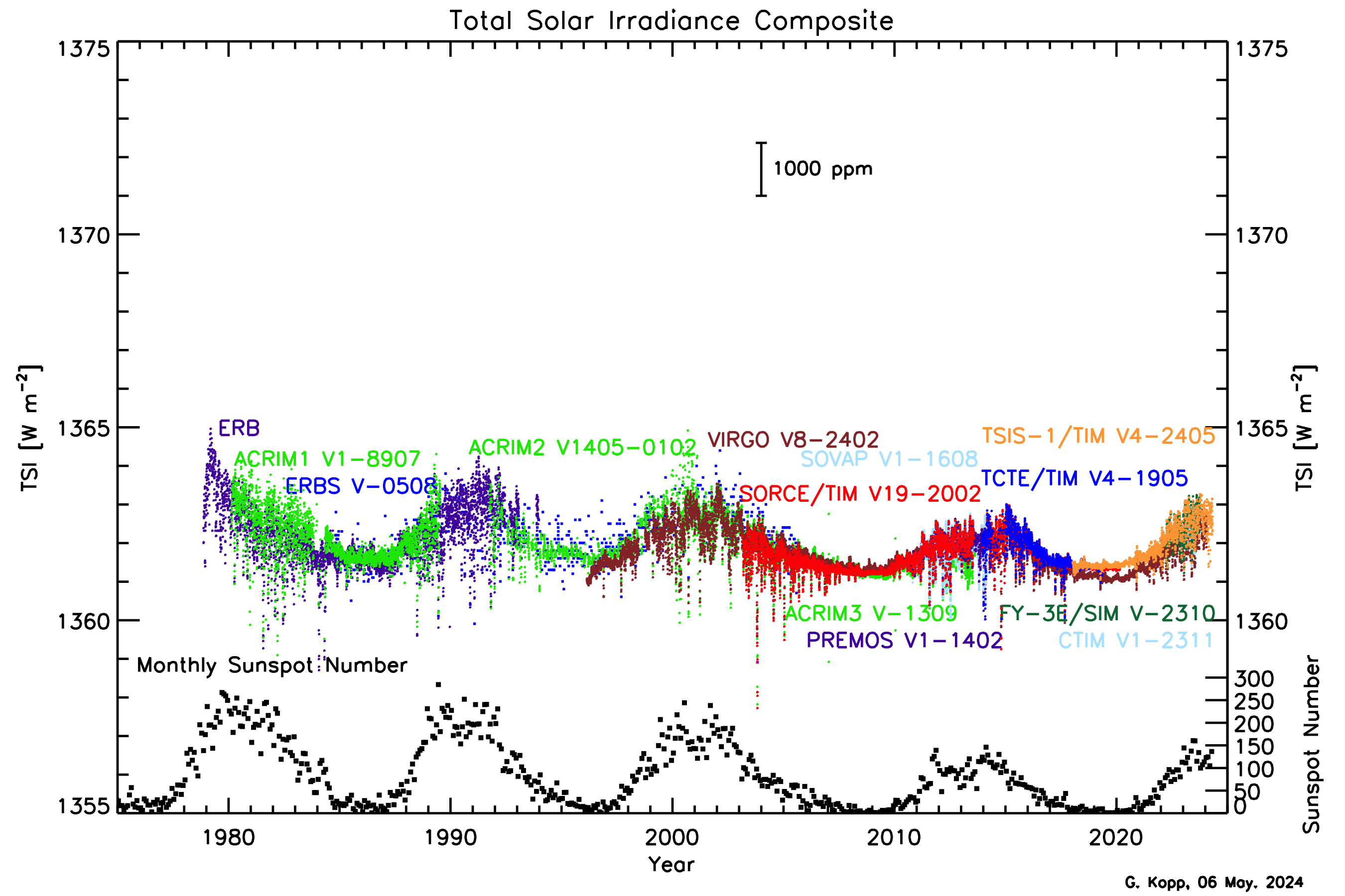
In the figure below, you’ll find TSI measurements from various satellites over the past few decades, alongside the number of sunspots. The two data sets correspond remarkably well—when we see an increase in sunspots, there’s a corresponding rise in solar radiation, and when sunspots are few, the TSI dips. By leveraging this relationship between sunspot numbers and TSI, scientists can actually reconstruct fluctuations in solar radiation going all the way back to the 1600s. This long-term reconstruction works similarly to how scientists reconstruct Earth’s temperature record, as we discussed earlier in this section, giving us deeper insights into how the Sun’s variability affects our climate over centuries.

In the figure above, you’ll notice a regular cycle in both TSI and sunspots, which occurs roughly every 11 years. The total amount of radiation the Earth receives from the Sun varies by about 0.1% between the high and low points of these cycles. If we take a longer view looking at sunspot numbers as far back as the 1600s in the figure below - we can see that these cycles have been repeating for a long time. In addition to the 11-year cycles, there are longer term fluctuations that occur over 80-90 years, known as Gleissberg cycles. Sunspot activity tends to be relatively low during certain periods, such as the early 1800s, early 1900s, and early 2000s, with higher activity occurring in between.

One particularly notable feature of the sunspot record is the pronounced absence of sunspots from 1650 to 1715, a period known as the Maunder Minimum. This era, named after British astronomers Edward and Annie Maunder, represents a time when the Sun's activity was unusually low. During this period, global temperatures were also lower, especially in the Northern Hemisphere, contributing to what is often called the "Little Ice Age." This wasn't a true ice age like we previously discussed, but it was a time marked by colder winters and significant climatic shifts in Europe and North America. Although the exact cause of this diminished solar activity remains a mystery, recent research by astronomers from Penn State (led by undergraduate-at-the-time Anna Baum!) has uncovered evidence of a similar phenomenon occurring in another star, offering intriguing clues about these solar mysteries.

Now, I want to stress that while the amount of radiation the Earth receives from the sun does change, this variability plays a relatively minor role in influencing the Earth's temperature. A quick back-of-the-envelope calculation on the effect of fluctuations in TSI (which I won't make you do, but meteorology majors study!) shows that the impact on the planet’s surface temperature is less than 0.1°C. Furthermore, we’ve been in a period of declining fluctuations in solar activity since the 1950s. These variations are also accounted for in climate models, where we can confirm that they play a minor role in driving changes in the Earth's temperature compared to other factors like greenhouse gas concentrations. So, when talking heads say, "climate change is just a bunch of sunspot cycles," they aren't totally wrong, but observed changes in the sun are a drop in the bucket compared to the temperature changes we are currently observing and expect to observe in the future.

Read...

Hopefully, I’ve convinced you that ongoing changes in the Sun’s output are relatively small (at least during human history). But before we move on, I want to point out something strange: scientists have discovered that when Earth first formed about 4.5 billion years ago, the Sun was much fainter than it is today. In fact, astrophysical models tell us that the Sun’s energy output was about 30% lower back then!

Check out the graph below. It shows the time-series of luminosity (i.e., emitted energy), radius, and temperature of the Sun over the past 4.6 billion years of its life—and it projects another 7 or so billion years into the future. The values on the y-axis are all normalized to present-day values, meaning a radius of 1.2 would mean the Sun is 20% larger than it is today. I want to emphasize that the x-axis is in billions of years, so all of human history is constrained to that small point where all three lines cross 1.0. (None of us will be around—barring some serious medical breakthroughs—to experience much beyond that!) 

If you’ve taken an astronomy class, you might have learned that the Sun is continually growing larger (as this graph shows!). But for this class, we’re just focused on energy, so pay attention to the luminosity (the red curve). For the first two billion years of Earth’s life (note, Earth formed about 60 million years after the Sun’s birth), the energy the Sun output was less than 80% of what it is today. This means early Earth should have been much colder—so cold, in fact, that it should have been frozen solid. Yet, we know from the proxy records we’ve discussed that liquid water existed on the surface, and life was already starting to take hold. In fact, things were quite warm! 

This puzzle is known as the Faint Young Sun Paradox—how did Earth stay warm enough to support life when the Sun wasn’t as bright? Astronomers Carl Sagan (you have probably heard of him, or at least heard of "The Pale Blue Dot") and George Mullen first raised this question in 1972. So, what could have kept Earth warm enough to sustain liquid water and life? Scientists aren’t 100% sure, but the most widely accepted theory involves greenhouse gases. 

When Sagan and Mullen first introduced the Faint Young Sun Paradox, they suggested that high concentrations of ammonia gas (NH₃) could have been responsible for keeping Earth warm. We haven’t talked much about ammonia because—well—there isn’t much of it in the atmosphere today! But it is an effective greenhouse gas, meaning it can trap heat in the atmosphere, much like carbon dioxide (CO₂). However, there’s a catch: ammonia is easily destroyed by sunlight. Once exposed to ultraviolet radiation, it breaks down into nitrogen (N₂) and hydrogen (H₂) gases, which don’t trap heat as effectively. Although Sagan later suggested that a photochemical haze might have shielded ammonia from destruction, research eventually showed that this idea wasn’t plausible—the haze itself would have cooled Earth’s surface, counteracting any warming from ammonia. I mention this to highlight that even the most brilliant scientists aren’t always right! 

Greenhouse gases to the rescue?

So, if ammonia couldn’t do the job, what could? Most scientists now agree the answer is carbon dioxide. Remember when we first introduced the greenhouse effect? We explained that carbon dioxide is a potent greenhouse gas, and we’ll dive deeper into that next lesson. For now, the key takeaway is simple: more greenhouse gases = a warmer planet! CO₂ levels in Earth’s early atmosphere were likely much higher than they are today. 

Scientists have used models to estimate how much CO₂ would have been needed to keep Earth warm enough for liquid water during the Faint Young Sun period. These models suggest CO₂ concentrations could have been up to 1,000 times higher than present-day levels. Trust me, that’s a lot of carbon dioxide! This “supercharged” greenhouse effect would have compensated for the Sun’s dimmer output, allowing Earth to remain warm enough for water—and life—to exist. 

The figure below shows this tradeoff over time. In the early part of Earth’s history (on the left side of the graph), solar energy (brown curve) was much lower, but CO₂ concentrations (blue curve) were sky-high. As we move forward in time (left to right), the Sun’s brightness increased while CO₂ levels dropped—without this balance, Earth would have become too hot for life as we know it. 

But carbon dioxide wasn’t the only greenhouse gas at play. There’s also evidence that methane (CH₄), another potent greenhouse gas we’ll discuss soon, played a crucial role. Early Earth was home to a variety of microbes—single-celled organisms—that produced methane as a byproduct of their metabolism. These microbes were anaerobic, meaning they didn’t require oxygen to survive. In the oxygen-poor atmosphere of the time, they thrived, and their methane emissions could have significantly contributed to warming the planet. 

In the early 2010s, scientists analyzing ancient marine sediments found clues suggesting methane worked alongside CO₂ to keep early Earth warm. By pulling out ocean sediment cores, they discovered certain iron-rich minerals that coexisted during the early part of Earth’s history. This hinted at a balance between CO₂ and hydrogen (H₂) in the atmosphere, with methane playing a key role. Methane is far more effective at trapping heat than CO₂, so even small amounts could have had a big impact on global temperatures. 

Why is this important? 

The Faint Young Sun Paradox doesn’t just teach us about Earth’s distant past—it also highlights the incredible power of greenhouse gases. Even small changes in CO₂ and methane levels can dramatically impact the planet’s temperature. In other words, the lesson of the Faint Young Sun Paradox is clear: greenhouse gases matter—a lot! In fact, our planet has fundamentally relied on the balance between energy from the Sun and the Earth’s atmosphere to sustain life. If we could snap our fingers and put as much CO₂ into the atmosphere as there was during the early Earth’s history, we’d fry like an egg (well, eggs wouldn’t exist, I suppose…) 

 William Shakespeare once wrote in The Tempest, “What’s past is prologue.” He used the quote in the context of fate, suggesting that everything leading up to the present shapes what happens next. But we can also apply this to climate: history sets the stage for our present and future. Understanding the role of greenhouse gases in Earth’s climate system, both past and present, is key to anticipating the future of our planet.  

Read...

On June 15, 1991, Mount Pinatubo in the Philippines erupted in one of the most powerful volcanic events in recorded human history. In fact, it was the second-largest eruption of that century. Fortunately, there were warning signs before the eruption, and thanks to accurate forecasts from the Philippine Institute of Volcanology and Seismology and the U.S. Geological Survey, evacuation orders were issued in time. This likely saved more than 5,000 lives in the densely populated area around the volcano. When we think of volcanic eruptions, we often picture towering ash clouds, avalanches, and rivers of molten lava. But have you ever considered how such eruptions could affect the Earth's climate?

How Volcanos Impact the Earth's Climate

When a volcano erupts, it releases more than just dramatic ash clouds (see above) and lava flows—it also sends ash, dust, and gases high into the atmosphere. Heavier particles, like ash and fine rock, fall back to Earth relatively quickly, settling on the ground nearby. However, the smallest particles, especially those released in the most violent eruptions, can be injected high into the atmosphere and remain there for months, sometimes even longer. These fine particles, often in the form of aerosols, are carried by global winds, spreading around the Earth.

But that’s not all volcanoes release. Along with ash and dust, they emit a variety of gases, including water vapor, carbon dioxide (CO₂), and sulfur dioxide (SO₂). While water vapor and carbon dioxide are both well-known greenhouse gases that trap heat and contribute to warming the Earth’s surface, their effect from individual volcanic eruptions is actually quite small compared to human-driven emissions. Early in Earth’s history, when volcanic activity was much more frequent, these gases played a bigger role in shaping the planet’s climate. Today, however, the amount of carbon dioxide released during eruptions is minimal compared to the vast quantities emitted by human activities such as burning fossil fuels -- essentially just a rounding error in the carbon budget we'll talk about in the next lesson.

Sulfur Dioxide (S0₂)

Sulfur dioxide (SO₂), on the other hand, is particularly important. It plays a crucial role when it comes to volcanic impacts on the climate. When a volcano erupts, vast amounts of SO₂ can be ejected into the stratosphere. This is the atmospheric layer above the troposphere—well beyond where commercial airplanes fly. In the troposphere, rain can wash out particles fairly quickly, but in the stratosphere, where there is much (much) less condensed water, SO₂ can linger for months or even years. Once in the stratosphere, SO₂ reacts with the small amount of water vapor present to form sulfuric acid (H₂SO₄) aerosols. These tiny particles act like mirrors, scattering and reflecting incoming solar radiation away from the Earth’s surface, effectively increasing the planet’s albedo (I wasn't kidding when I said you'll see that word a lot in this class!). This reflection of sunlight causes a cooling effect on the Earth's surface, and after major volcanic eruptions, we can often observe noticeable dips in global temperatures. Scientists measure the amount of sunlight blocked by these aerosols using a metric called aerosol optical depth. This metric, commonly abbreviated AOD, is a gauge of how much sunlight is being scattered by particles in a given "column" of atmosphere.

The most violent eruptions can significantly impact the Earth’s climate, leading to rapid cooling followed by a slow recovery. The figure below shows notable volcanic eruptions over the past 150 years. What I've actually plotted is the stratospheric aerosol optical depth -- high values mean there are more particles in the stratosphere. Note the very strong linkage between when you see spikes in the data and volcanic eruptions, telling us that when we have lots of aerosols in the stratosphere, they were thrown up there by a big volcano.

Since these aerosols can increase planetary albedo, they can reduce sunlight reaching the surface and temporarily cool the planet. Historical temperature records reveal clear drops in global mean temperatures that align with major volcanic events. These cooling periods can last several years as the aerosols slowly dissipate from the atmosphere and the climate gradually returns to its previous state. The strongest volcanos may cool the planet up to 1°C, which is 10x more than the variability from sunspots we learned about! But I should emphasize that these effects are transient -- once all the aerosols "fall out" of the atmosphere, it's like the volcano no longer exists, so they don't do anything to stop or reverse long-term trends. While volcanic cooling is a natural process, it underscores the Earth’s sensitivity to changes in atmospheric composition, even for relatively short periods.

Read...

Summary

What did we learn?

• Climate proxies are natural recorders of past climate, helping scientists reconstruct conditions long before modern instruments existed. Key proxies include:
  • Ocean and lake sediments: Layers of sediment provide clues about past water temperatures and ice coverage.
  • Ice cores: These trap ancient air bubbles, revealing past greenhouse gas levels and precipitation patterns.
  • Tree rings: The width and density of rings reflect yearly climate conditions like temperature and rainfall.
  • Pollen grains: Found in sediments, they indicate the types of plants present, which helps infer past climate conditions.
• Proxies tell us that the Earth’s temperature has varied significantly over its 4.5 billion year lifespan.
• Orbital parameters are long-term cycles that influence Earth's climate by changing how much sunlight reaches different parts of the planet:
  • Obliquity (tilt): The angle of Earth's axial tilt changes over a 41,000-year cycle, affecting the intensity of seasons. Greater tilt leads to more extreme seasonal differences, while a smaller tilt reduces seasonality.
  • Precession (wobble): Earth’s axis wobbles like a spinning top, altering the timing of seasons relative to Earth's position in its orbit. This cycle takes about 19,000 to 23,000 years.
  • Eccentricity (orbit shape): Earth’s orbit changes from more circular to slightly elliptical over a 100,000-year cycle, impacting the distance between Earth and the Sun, contributing to glacial-interglacial cycles.
• Ice-Albedo Feedback: A positive feedback loop where ice and snow reflect sunlight, cooling the Earth. As the planet cools, more ice forms, increasing reflectivity and further lowering temperatures. Conversely, when ice melts, less sunlight is reflected, warming the planet and accelerating ice loss. This feedback plays a crucial role in amplifying temperature changes during glacial and interglacial periods.
• Sunspots: Dark, cooler areas on the Sun’s surface that appear in cycles, typically every 11 years. While sunspots emit less energy, the surrounding areas (faculae) emit more, leading to slight variations in the Sun’s total energy output. These cycles can influence short-term climate patterns but have a relatively minor impact on long-term global temperatures compared to greenhouse gases.
• We learned about the Faint Young Sun Paradox. Despite the Sun being about 30% dimmer when Earth first formed, the planet remained warm enough to support liquid water and early life. This paradox is likely explained by much higher concentrations of greenhouse gases like carbon dioxide and methane, which trapped more heat and offset the Sun's weaker output.
• Volcanoes: Large volcanic eruptions release sulfur dioxide into the stratosphere, where it forms reflective aerosols that block sunlight and cool the Earth temporarily. These cooling effects can last for several years, with major eruptions like Mount Pinatubo in 1991 causing global temperatures to drop by up to 1°C. However, volcanic impacts are short-term and don't offset long-term warming trends.

Now that we’ve explored the natural processes that influence Earth's climate over time, it’s important to understand how human activities are accelerating climate change. In the next section, we’ll dive into the science behind anthropogenic climate change and examine how greenhouse gas emissions are driving rapid warming in recent decades.