Read...

When you visit the hospital, one of the first things that is done is checking your vital signs. These “vitals” are medical measurements that provide data about the body's basic functions and include heart rate, blood pressure, oxygen levels, etc. They are important because they give a quick picture of a patient’s overall health, aid in the detection and treatment of health problems, and guide future medical decisions.

Similarly, in our exploration of Earth's climate system, we need to select measurements that allow us to view the basic state of the climate and how it behaves, changes, and impacts our planet. This set of simple, but very important, parameters is known as Essential Climate Variables, or ECVs.

An ECV can be defined as a physical, chemical, or biological variable that holds a key importance in characterizing Earth's climate. ECVs are the variables that scientists believe are crucial to monitor because of their profound influence on the global climate system and their importance in understanding climate change. Moreover, these variables are pivotal in assisting decision-making processes related to climate change adaptation and mitigation.

There are three main criteria that make a particular measurement an ECV:

1. Relevance: The variable is critical for characterizing the climate system and its changes.
2. Feasibility: Observing or deriving the variable on a global scale is technically feasible using proven, scientifically understood methods.
3. Cost-effectiveness: Generating and archiving data on the variable is affordable. It mainly relies on coordinated observing systems using proven technology, taking advantage of historical datasets where possible.

While relevance and feasibility seem obvious, I want to emphasize that cost-effectiveness is also extremely important. ECVs require us to get as holistic of a view of the entire Earth system as possible – if we design a drone that can measure temperatures far higher than where planes fly, but the cost is $10 billion per craft, that doesn’t do us a tremendous amount of good in terms of sampling the entirety of the planet!

While we could probably think of some ECVs right off the top of our heads (surface temperature, anyone?), we delegate the organization of them to the Global Climate Observing System (GCOS). GCOS operates under the sponsorship of the World Meteorological Organization (WMO), the Intergovernmental Oceanographic Commission (IOC) of UNESCO, the United Nations Environment Program (UNEP), and the International Science Council (ISC). Phew, don't worry; there will not be a quiz on any of *those* acronyms!

So, what are some examples of ECVs?

We can consider that this list of ECVs provides the foundation for sharing climate data worldwide, both for current conditions and historical records. It is a Rosetta Stone that allows researchers from all around the world to speak the same climate language. However, I should emphasize that these variables – while we’ll use them a lot this semester – are not an “end-all be-all.” Scientists use a host of other data to track the climate system, too. We should just think of these 50 ECVs as a starting point for more complex climate studies. We also shouldn’t necessarily consider a single variable on this list to be more important than another; they all play a crucial role in different ways in understanding Earth's climate system as a whole.

Atmospheric

Atmospheric variables are probably the ones you are most familiar with. These even include those traditionally used to describe weather on your 6 PM news, like precipitation, wind, temperature -- even lightning. The atmospheric domain is divided into surface (near-ground) and upper air measurements (think about all the space above a tall skyscraper). Scientists are also concerned with air's chemical makeup. Pay special attention to the Earth’s “radiation budget,” which we'll discuss soon. This, in conjunction with the variables defined by atmospheric composition, is what is keenly important for understanding how our climate has changed and may change in the future.

Land

ECVs taken on land may seem diverse, but elements like river discharge and leaf area index are connected. Both contribute to energy and mass exchange on land surfaces. Other variables like soil carbon and fire disturbances relate to the global carbon cycle. Human activities can impact soil carbon levels, and fires, whether natural or human-caused, release significant carbon into the atmosphere. Of course, it goes without saying that we – as humans – live on the land’s surface, so these ECVs are of particular importance in our day-to-day lives. How much snow is on the ground can be pretty important in what we do on a dreary day in December!

Ocean

Lastly, in the ocean, things look a little different. Yes, we still look at temperature and currents (the ocean equivalent of wind), but we also look at ocean water composition, including salinity, acidity, oxygen levels, and tracers. Tiny organisms like phytoplankton help absorb carbon dioxide from the atmosphere and produce oxygen. By monitoring these ocean variables, we can learn a great deal about the evolution and vulnerabilities in specific ecosystems.

Defining ECVs is only half the story -- how do we go about measuring them? We really have two options, read on to learn about what each of these are.

Read...

In-situ measurements of the land and atmosphere

In-situ measurements require that the instrumentation be located directly at the point of interest and in contact with the subject of interest. For those who took Latin in high school, you may remember that “in situ” means “in position.” Going back to our vital signs analogy from before, this would be the equivalent of a thermometer that was placed under your tongue. Measuring the air temperature with a thermometer is the easy climate analog – we are physically measuring the temperature at a specific location, but having the air make direct contact with the thermometer gives us our reading. The same thing holds for taking wind measurements (wind striking an anemometer or wind vane) or measuring precipitation (rainfall falling into a rain gauge).

A great deal of our in-situ measurement toolbox centers on the land surface, where humans live. As implied before, one of the most important ECVs for studying climate is near-surface temperature. This is the temperature outside that you and I experience at any given time, and is the temperature we are all familiar with being reported by our local weather forecasters. It is inexpensive to measure, many of you may already do this, and is almost always reported from a surface weather station, whether those be at airports or in backyards.

Thermometer records from weather stations, islands, and ships provide us with more than a century of reasonably good global estimates of surface temperature change. Measurements were historically made using mercury or alcohol thermometers, which were read manually and recorded by hand at either specified intervals or just when convenient. Over the past few decades, these observations are increasingly made using electronic sensors that transmit data without the need for human intervention. Heck, even things like your car and smartphone likely have the capability to measure temperature automatically! Some regions, like the Arctic and Antarctic, and large parts of South America, Africa, and Eurasia, have not been as well sampled over the past century or so, but records in these regions become more available as we moved into the mid and late 20th century.

These data can be reported as a time series as we discussed in the previous lesson but given that we are interested in the surface temperature and how it has evolved over the last ~200 years, we typically take these temperatures, scattered at various points and times, and merge them into a single organized dataset that can be visualized as a map. A key benefit to this approach is it reduces the potential impacts of outliers and bad data while giving us a “global” view of the planet. The figure below shows the result of this as derived by the Berkely Earth project. The scientists working on the dataset have merged all in-situ surface temperature observations from 2022 and then compared that result to the 1951-1980 global average.

2022 surface temperature anomaly map as synthesized by the Berkeley Earth project. The map is generated by statistically merging all the surface observations taken over 2022 and comparing them to the reference data period from 1951-1980.

Credit: Global Temperature Report for 2022, Berkeley Earth is licensed under CC BY-NC 4.0 International

Moving one step further, all of these data points and different locations and times can be merged together to form a single global mean. This is the value that is frequently seen in the media or other outlets when discussing climate change over the past hundred years. Note that there is not one specific way to calculate a single global mean – see the graph below, which shows six different time-series of the global mean temperature anomaly! It’s important to note, however, that while the lines differ slightly even though they are generally using the same observational record, the overall behavior and trends of the curves are very similar, no matter which strategy is employed.

A time series of merged surface temperature anomaly observations starting from 1850. The anomalies are relative to (or deviations from) surface temperatures averaged from 1850-1900. Each color denotes a different way of calculating the global mean surface temperature from observations.

Credit: Global Mean Temperature Compared to 1850-1900 Average, World Meteorological Organization, CC BY-NC-ND 4.0 DEED

Read...

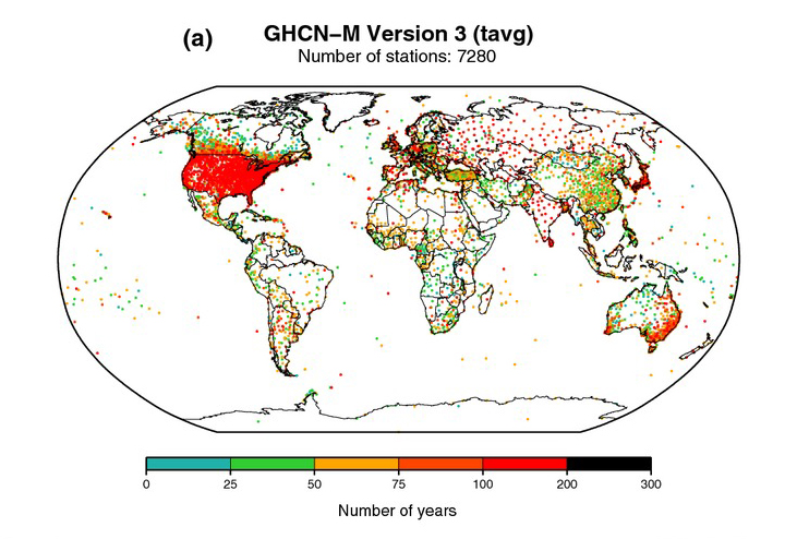
We’ll see later that the ocean is a key component of the climate system, particularly on longer timescales. But in the last section, we noted that most of our in-situ measurements of the climate system are taken on the land surface. In fact, see the below figure, which shows where each of the 7280 stations that go into the Global Historical Climatology Network dataset is located. We see a ton of red dots over the United States, Europe, Japan, and parts of Australia, indicating dense, long-term records. We see a growing network elsewhere around the world, but predominantly focused on land. Many fewer points are out over the ocean – these may be small islands, ships, oil rigs, or other buoys, but since humans don’t generally live in the water, observations there are far trickier!

Station locations which are included in the 3rd version of the Global Historical Climatology Network dataset. The color corresponds to the number of years of data available for each station.

Credit: Figure 1, by J.J. Rennie, Geoscience Data Journal

So how do we measure ocean properties from an in-situ perspective? While we have some measurements of surface ocean temperature from ships (throw a bucket overboard, pull up some water, take the temperature!), a larger view of ocean variables didn’t come until the widespread use of buoys, which occurred during the middle of the 20th century. Surface weather buoys (either anchored or drifting) are primarily used to help with weather forecasting but can also aid during emergency responses to chemical spills, provide engineering baselines for wind farms, and other cool applications. But while not designed for climate modeling, we can take advantage of this network and use their observations in our dataset as well. There are a few problems with relying on this buoy network. The first, and perhaps the most obvious, is that they do not have nearly the same spatial coverage that measurements taken on land have. Below is a snapshot of buoys cataloged by NOAA’s National Data Buoy Center on a given day. Look at all those gaps!

Locations of buoys tracked by NOAA’s National Data Buoy Center on October 19th, 2023. Yellow dots mean buoys that have actively reported in the past 8 hours. Red dots mean possibly active buoys, but ones that haven’t reported recently. Orange dots indicate inactive buoys that offer historical data.

Credit: Station ID Search, National Data Buoy Center, National Oceanic and Atmospheric Administration (NOAA) (Public Domain)

For the record, the buoys (or oil-drilling platforms) marked with yellow dots are stations that have recorded data recently. Meanwhile, stations marked by red dots are still considered active but hadn't reported data in at least eight hours at the time this image was produced. Orange dots represent buoys that used to exist but are no longer active. For example, the rightmost buoy on the plot -- the one in the Red Sea -- was maintained by the King Abdullah University of Science and Technology, which shared its data with NOAA. However, those reports stopped in 2010. While the coastline of the United States and the central Gulf of Mexico are well sampled by buoys and observations from oil-drilling platforms, farther out over remote ocean waters, a tropical cyclone finding a buoy is akin to finding a needle in a haystack. The buoys over the Atlantic and other oceans around the world are widely spaced, leaving huge gaps between buoy observations.

The second challenge is that they tend to measure basic surface variables of the ocean, such as sea surface temperature. This only gives us a small glimpse.

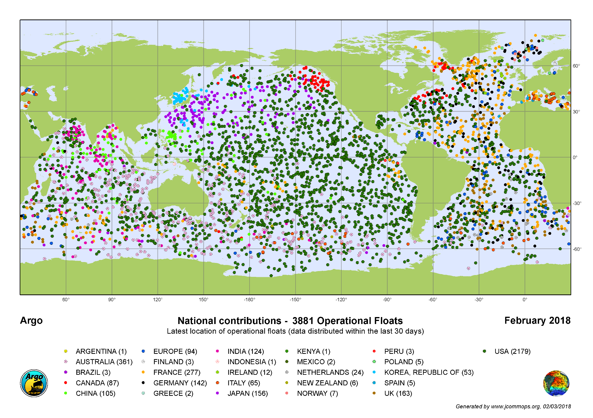
There are efforts to address these gaps. Perhaps the most notable is Argo, an international program that uses profiling floats to observe temperature, salinity, and currents. The unique feature of Argo floats is that they move up and down in the ocean according to a set schedule. To do this, the floats adjust their density by altering their volume by pushing out mineral oil and expanding a rubber bladder at its lower end. This expansion makes the float less dense than the surrounding seawater, causing it to rise. At the surface, they transmit all the measurements they have taken over the past ten or so days at depths as deep as 2,000 m. After reporting, the float contracts the bladder, reducing its volume and increasing its density, which allows it to descend back into the depths.

Currently, there are roughly 4,000 floats producing 100,000+ temperature/salinity profiles per year. This may seem like a lot but check out the picture below – there remain large gaps in ocean observations that can be as wide as the distance from Miami to New York City. Further, many portions of the ocean are far deeper than 2000m. New technology allows a small subset of these floats to go down to 6000m depth, which is still only approximately half as deep as the deepest part of the ocean (the Challenger Deep). Clearly, there is still a great deal of room for improvement in our in-situ ocean observing network!

National Contributions - 3881 Operational Floats. Latest location of operational floats (data distributed within the last 30 days) February 2018

Credit: Argo float data visualization, Argo (Public Domain)

Read...

Low-Earth and High-Earth Orbits

Satellites orbit Earth at various altitudes, each serving specific functions. The two most relevant for climate science are “Low-Earth orbits” and “High-Earth orbits.”

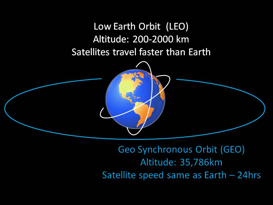
Low-earth orbits, which range from approximately 160 to 2,000 kilometers above Earth's surface, are critical for various applications, including Google Earth imagery. For climate observations, many of these satellites follow "polar" orbits, circling over both the north and south poles multiple times daily -- see the figure below for an idea. In fact, because they track over these high-latitude regions, we generally call these satellites "Polar Orbiting Satellites." These satellites complete an impressive 14 orbits daily while Earth rotates beneath them. Their orbits are consistent, forming a stable "highway" in space, allowing them to capture images of different locations on Earth as our planet continues its constant rotation beneath their path.

While polar orbiting satellites in low-Earth orbits are vital for capturing detailed global snapshots, high-Earth orbits offer a different perspective. Satellites in high-Earth orbits, often referred to as "geostationary satellites," remain fixed over a single point on the equator, providing continuous monitoring of specific regions. This contrast between low-Earth and high-Earth orbits is key to understanding their complementary roles in climate observation!

Polar Orbiting Satellites

So, polar orbiters get a worldly view, but not all at once! Like making back-and-forth passes while mowing the lawn, these low-flying satellites methodically scan the Earth in swaths about 2600 kilometers (1600 miles) wide, covering the entire globe twice every 24 hours. Each pass collects a narrow strip of data as the satellite moves along its orbit, building a complete picture of the Earth's surface over time. The appearance of a narrow swath against a data-void, dark background on a satellite image is a dead giveaway that it came from a polar orbiter. This characteristic pattern is a direct result of the satellite's polar orbit, which allows it to capture data from pole to pole as the Earth rotates beneath it. For example, see this animation below. Just like mowing a lawn, the satellite continuously orbits over the top and bottom of the planet, taking row after row of pictures with each pass! As it progresses, the satellite methodically pieces together a comprehensive view of the Earth's surface, ensuring that every part of the planet is eventually imaged, albeit not simultaneously.

Video: Polar Orbiting: NOAA-17 Satellite Coverage (0:30) (No Audio)

Read...

When considering the pursuit of a robust climate record, the strategic use of both types of satellites proves highly beneficial. Geostationary satellites excel in monitoring specific regions with exceptional temporal persistence, while polar orbiters offer the broader perspective necessary to capture global climate trends and changes. The combination of these two satellite types complements each other's strengths and is instrumental in advancing our understanding of Earth's climate system!

A major hurdle in the realm of climate observation through satellites is their finite lifespan. On average, polar-orbiting satellites typically operate for approximately 5 to 10 years, while geostationary satellites often endure for roughly twice that duration. This poses a couple of significant challenges.

First, securing continuous financial resources – either from the governmental or private sectors -- becomes a critical imperative. Given the limited operational lifespan of satellites, ensuring sustainable funding for the ongoing replacement of these crucial instruments is essential. The maintenance of a robust satellite network hinges on the consistent investment required to effectively sustain climate monitoring endeavors and launch new and improved technology as warranted.

Secondly, the meticulous comparison of observations between different satellites demands careful attention. Satellite instruments are inherently diverse, and variations in calibration errors can exist between them. These discrepancies present challenges when striving to make accurate and seamless comparisons between observations collected by distinct generations of satellites. This is particularly vital when tracking ECVs. To understand the precision required in ECV data, satellite instruments must exhibit the capability to discern subtle atmospheric temperature trends, as minuscule as 0.10 degrees Celsius per decade. Likewise, they should possess the sensitivity to track ozone changes as minute as 1% per decade and variations in the sun's output as diminutive as 0.1% per decade. These exacting requirements underscore the importance of precise instrument calibration and meticulous data analysis to ensure the accuracy of climate observations over the long term.

An example of this “dance” is two recent NASA satellites used to measure precipitation: GPM (Global Precipitation Measurement), and TRMM (Tropical Rainfall Measuring Mission). TRMM was launched in 1997 and orbited in faithful service until 2015. When TRMM grew close to the end of its useful lifetime, GPM was funded by NASA and launched in 2014 with new instruments. Behind the scenes, the transition required an entire team solely dedicated to helping calibrate its observations so that they matched up with TRMM and that the observations from the two satellites could be glued together in time to teach us how precipitation has evolved over the past 30 years.

In addition to the satellites themselves, scientists develop data processing systems to “merge” multiple dataset sources together. We briefly touched on this above with in-situ observations, but naturally, you could easily imagine merging both multiple in-situ datasets with multiple remote sensing datasets! One such example in the U.S. is CMAP, which stands for the CPC Merged Analysis of Precipitation. CPC is an acronym for the Climate Prediction Center, the arm of the U.S.’s National Weather Service tasked with real-time monitoring of global climate and predictions of climate variability. After synthesis, such products allow us to create figures like the January mean precipitation climatology shown below. We arrive at a spatiotemporally continuous map of precipitation – “spatiotemporally continuous” means we can find a data point for any geographic location (spatio-) and any time (-temporal) as long as it’s contained in the dataset. Note the higher average precipitation totals in warm tropical regions, both over the ocean and in areas such as the Amazon rainforest, but some very dry areas in the subtropics such as the Saharan desert in Northern Africa. We’ll talk about the hydrological cycle and general circulation of the atmosphere later in the course to help explain why these patterns emerge.

Average January precipitation rate produced from CMAP data. Units are in mm/day.

Credit: CMAP: CPC Merged Analysis of Precipitation, National Center for Atmospheric Research (NCAR), is licensed under the Digital Millennium Copyright Act of 1998

Read...

You may have heard the term “big data” thrown around. You may even be currently majoring in something focused on data analytics or figuring out strategies to solve the “big data” problem. But what do we mean by “big data?” For simplicity, big data refers to extremely large and complex datasets.

Well, in many ways, climate data is just that! The National Centers for Environmental Information (NCEI) currently houses (as of 2023) more than 60 petabytes (1 petabyte = 1,000,000 gigabytes) of climate information. For context, an entry-level iPhone holds approximately 128 gigabytes of data – I would need more than half a million iPhones dedicated to storing climate data to hold it all! Another analogy is 60PB is equal to 5,268.704 years scrolling through tiktok assuming each video is around 13 MB and you watch around 100 tiktoks per hour. Remember, climate is the synthesis of weather, so to develop a solid climate record we effectively need to maintain logs of everything that has happened daily in perpetuity!

So, how do we do that here in the United States? Well, currently, if you want to use climate data in your day-to-day work, the best place to head is the National Centers for Environmental Information (NCEI), which is housed in Ashville, NC. NCEI (formally the National Climate Data Center) arose from a federal mandate way back in 1951. Before then, weather and climate archives were scattered at various offices around the United States. They were occasionally employed for regional analysis but without any national (or international) organization. It became clear to the federal government that coordination and standardization of such data was important to a variety of sectors around the country and was rapidly growing more important as interstate commerce was the norm rather than the exception.

The NCEI has evolved throughout the years. Data that were once handwritten on slips of paper were moved to punch cards, then cassette tapes and floppy disks, then optical media and hard drives. However, NCEI's primary goal has remained to safeguard these data and make it accessible to various stakeholders, including the public, businesses, government agencies, and researchers.

The user base for NCEI data spans a wide spectrum of sectors, including agriculture, air quality, construction, education, energy, engineering, forestry, health, insurance, landscape design, livestock management, manufacturing, national security, recreation/tourism, retailing, transportation, and water resources management. Climate underlies nearly every facet of our lives.

While the NCEI serves as a central brain for the U.S.’s climate data, other climate centers across the U.S. collaborate with it to manage more regional impacts of climate. There are six major climate centers around the country. All are affiliated with major research universities and help catalog and analyze climate data specific to their respective locations. These centers often foster collaborations between service climatologists and related academic disciplines, facilitating important ongoing research. These centers also contribute to important published releases, like the National Drought Monitor which you have almost certainly seen during a particularly dry spell. Since these regional centers focus on smaller service areas compared to NCEI they can more efficiently engage in public outreach and interact with and educate local communities.

A map denoting the six regional climate centers and which states they oversee. The stars denote the headquarters of each climate center, generally at universities with meteorology or climate science departments.

Credit: Regional Climate Centers, National Centers for Environmental Information (NCEI), (Public Domain)

Another relevant role linked to regional climate centers is that of the state climatologist. Some state climatologists are associated with regional climate centers, while others hold dual appointments as university faculty or government officials. State climatologists serve as experts to state governments and residents. As of 2013, there were 47 official state climatologists nationwide, including one in Puerto Rico – their primary roles are to collect and interpret climate data for their home state and disseminate climate data and information through various means.

Meet your state climatologist!

Kyle Imhoff joined the Pennsylvania State Climate Office in August 2011 and became Pennsylvania State Climatologist in July 2016. Kyle is a research assistant and instructor at Penn State University. He teaches courses in weather forecasting and applied climatology, and his research interests include applied climatology, synoptic meteorology, numerical weather prediction, and weather risk. Kyle also serves as the local manager for the Penn State team in the WxChallenge national collegiate forecasting competition. Kyle is currently a member of the American Association of State Climatologists.

Prior to joining the Climate Office team, Kyle focused on weather forecasting and assisted in producing winter weather forecasts for the Pennsylvania Department of Transportation in District 2. Kyle also worked as a research assistant at the University of Alaska Fairbanks in the summer of 2010 where he studied marine boundary layer cloud evolution.

Kyle was born and raised in Pennsylvania. Currently, he resides in Bellefonte, but his hometown is in Rockwood, Pennsylvania. While at Penn State, Kyle majored and earned his B.S. and M.S. degree in Meteorology.

Read...

You might be thinking, “How can it be that we seem to have so much data, yet not enough at the same time?” The reality is, we’re still far from having a highly detailed map of surface observations to study climate in the United States. Surface observations are usually taken near airports or in major cities, which means rural areas, suburbs, and other less populated regions are often overlooked in our climate-observing network. To close those gaps, scientists have started leveraging something called “citizen science.” Citizen science is the practice of public participation and collaboration in scientific research to increase scientific knowledge. This means that anyone—even you—can become a climate observer! With some basic training and simple instruments, the general public is asked to report what’s happening in their own backyard once a day. Of course, there are exceptions for vacations or school—after all, these observers are volunteers! A great example of this is The Community Collaborative Rain, Hail, and Snow Network, or CoCoRaHS.

CoCoRaHS was created to fill the gaps left by traditional weather stations. It’s a community-based network that relies on volunteers from all walks of life to measure and report precipitation in their areas. This approach provides a more complete picture of precipitation patterns across the country, making the data more reliable and useful for everyone.

Map of precipitation patterns across the country.

Credit: 24-hour precipitation map by NOAA/CoCoRaHS (Public Domain)

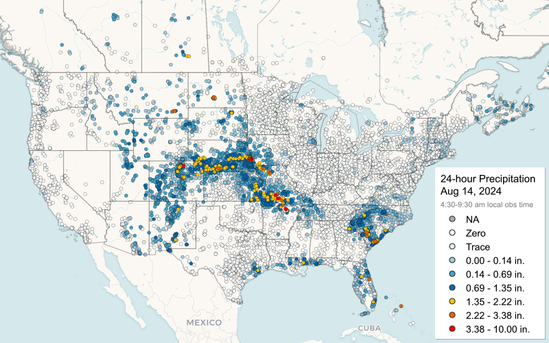
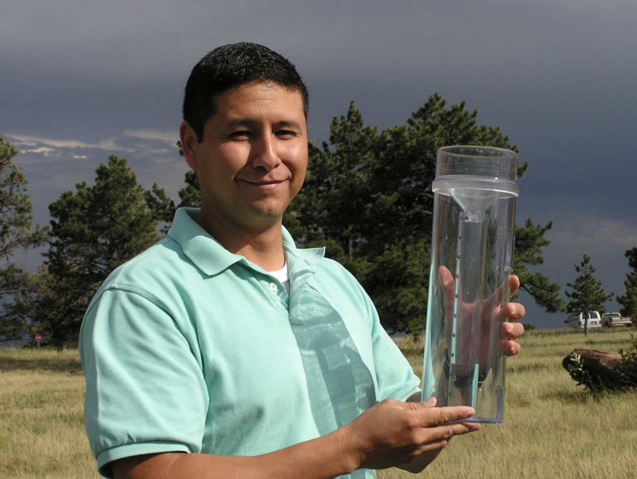
The origins of CoCoRaHS trace back to a catastrophic flash flood that hit Fort Collins, Colorado, in July 1997. A powerful, localized storm dumped over a foot of rain in just a few hours, causing $200 million in damages and claiming five lives. The existing weather stations didn’t capture the storm’s intensity because they were too far apart, highlighting the need for a more comprehensive and localized observation network. In response, CoCoRaHS was established in 1998 to improve the mapping and reporting of such extreme weather events. Since then, it has grown from a local initiative to a nationwide—and now international—network, providing critical climate data that benefits not just the United States, but other countries as well. Participation in CoCoRaHS is open to anyone, whether you live in a busy city or a quiet rural area. The process is simple: volunteers use straightforward, high-quality rain gauges to measure precipitation. With just a few minutes of effort each day, you can contribute valuable data that helps scientists and policymakers make informed decisions about water resources, agriculture, and disaster preparedness.

To ensure the data’s accuracy, CoCoRaHS offers comprehensive (and free!) training on everything from setting up your rain gauge to accurately measuring and reporting your observations. This training is crucial because consistency and precision are key to producing useful scientific data. Whether you’re reporting a quarter inch of rain or a major snowstorm, your contribution is significant.

A CoCoRaHS volunteer with his rain gauge.

Credit: CoCoRaHS Volunteer by NOAA/CoCoRaHS (Public Domain)

The data collected by CoCoRaHS volunteers are made available online almost instantly. You can even see your own house on the CoCoRaHS map! But more importantly, these data are used by scientists, resource managers, and decision-makers to gain a highly detailed and accurate understanding of precipitation patterns.

Being part of CoCoRaHS isn’t just about collecting data; it’s about joining a community of citizen scientists. It’s a practical, engaging way to connect with the weather and contribute meaningfully to your community. CoCoRaHS also offers webinars, training materials, and other resources to help volunteers deepen their understanding of weather and climate.

So, if you’ve ever wondered how much rain fell in your backyard—or if you just like the idea of contributing to real-world science—consider joining CoCoRaHS. It’s a small commitment that can have a big impact, and you might be surprised at how much you learn along the way.

Read...

Summary

• Essential Climate Variables (ECVs) are critical variables whose measurement helps scientists monitor and understand climate behavior, changes, and impacts, much like vital signs in human health. They are chosen based on relevance, feasibility, and cost-effectiveness, ensuring they provide key insights into the global climate system.
• Examples of ECVs include atmospheric variables (temperature, precipitation, wind), land variables (soil carbon, river discharge, leaf area index), and ocean variables (sea surface temperature, salinity, phytoplankton). The Global Climate Observing System (GCOS) organizes these to provide a standardized framework for global climate data collection and sharing.
• In-situ measurements involve collecting data directly from the point of interest, such as using thermometers for temperature or rain gauges for precipitation. They provide reliable data but can be limited by geographic coverage, especially over oceans.
• Ocean measurements often rely on buoys and ships but are supplemented by the Argo program, which uses floats to measure temperature and salinity at various depths. Despite the network of about 4,000 floats, gaps remain, especially in remote ocean areas and deep ocean zones.
• Remote sensing via satellites allows for continuous global monitoring of ECVs. Polar-orbiting satellites provide detailed snapshots of different Earth regions, while geostationary satellites monitor the same area continuously. Both types are essential for a comprehensive climate record.
• The National Centers for Environmental Information (NCEI) manages U.S. climate data and collaborates with regional centers to support research, public outreach, and informed decision-making.
• Citizen science initiatives like CoCoRaHS involve volunteers reporting local precipitation to fill gaps in traditional climate observation networks, enhancing data coverage and accuracy.