Understanding Distributions

Read...

There are three types of distributions we’ll primarily use this semester.

Uniform Distribution:

In a Uniform Distribution, every value in the dataset has an equal likelihood of occurring. On a graph, this is represented graphically as a flat, horizontal line. This distribution is characterized by the minimum and maximum values of the distribution. The probability of any given value occurring within this range is constant, and values outside of this range have a probability of zero. For example, in our dice example above, when rolling a single die, the odds of rolling one single number are equally likely, between 1 and 6, demonstrating a uniform distribution.

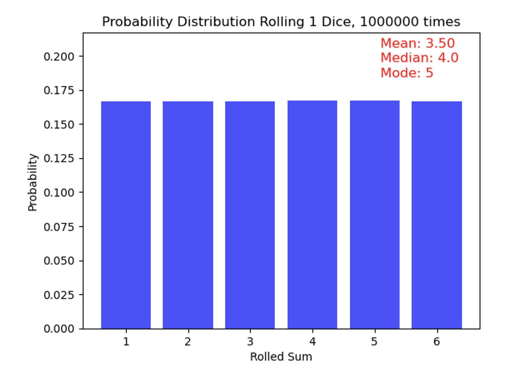
Eagle-eyed observers might take note of the statistics in the top-right corner of the figure, which show a mean of 3.5 (as expected), a median of 4, and a mode of 5. Wait—those bars look flat, so how is the mode 5!? These small deviations from perfect uniformity arise because the distribution is based on a finite (though large) sample of rolls rather than an infinite one. To make this clearer, I have added the number of rolls for each outcome above the bars, highlighting these slight differences even though the overall distribution appears very flat. With truly infinite rolls, the median would settle exactly at 3.5, and no single number would stand out as the mode.

Normal Distribution:

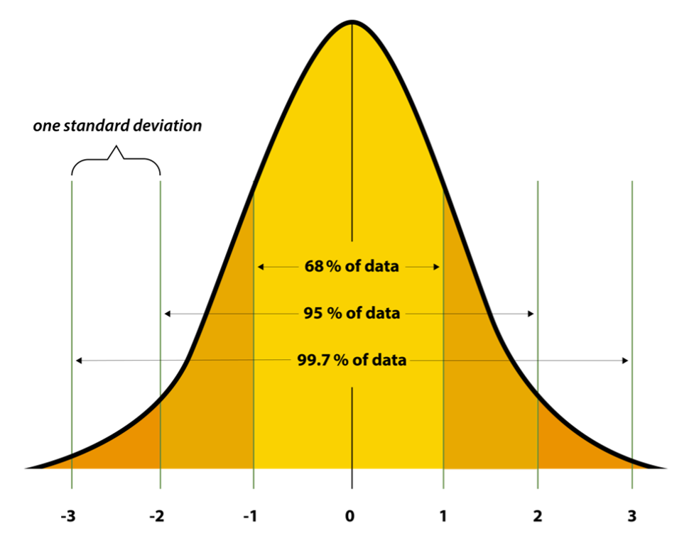
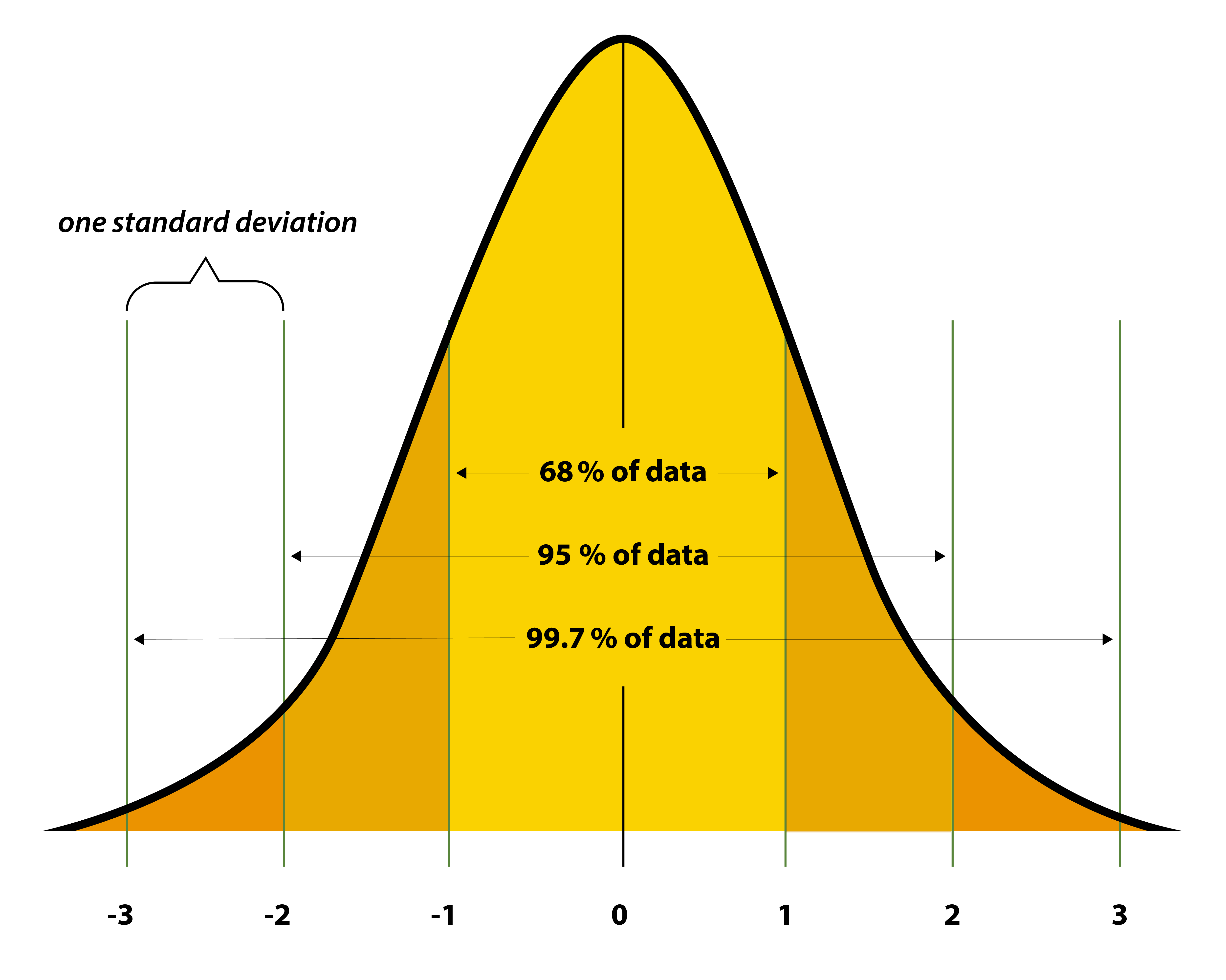
Uniform distributions are simple, but quite rare in nature. A common distribution seen in climate science – and quite prevalent across natural phenomena -- is the Normal Distribution, sometimes known as a Gaussian Distribution. This distribution follows a “bell-shaped” curve, with values closer to the central tendency (the mean and median!) being far more likely to occur than values in the “tails” of the distribution (very warm or very cold temperatures, for example). We also can briefly introduce the idea of “standard deviation” which is a measure of how much variation exists within a dataset. It is usually denoted by the Greek letter sigma. You may recognize these values, since some professors will “curve” their class grades based on this distribution (but not this one!). Small standard deviations tell us the distribution is very narrow, and all values tend to fall very close to one another. Large standard deviations tell us the opposite. If you are in a class where the mean on an exam was 81, and the standard deviation was 2, this means a *lot* of people scored very close to 81! On the other hand, if you have a mean of 81, but a standard deviation of 15, it means the distribution was far more spread out. In a symmetric normal distribution, about 68% of the data falls within one standard deviation of the mean, 95% within two standard deviations, and 99.7% within three standard deviations. Sometimes, you will hear people refer to something as a “three-sigma” outcome – this comes up in all walks of life, not just climate science. It means that it’s an event that falls at or outside the three standard deviation limit. If 99.7% of events fall within 3 standard deviations, it means a three-sigma events has less than a 0.3% chance of occurring in your distribution. Let's consider the IQ scores of a population, if IQ scores follow a normal distribution with a mean of 100 and a standard deviation of 15. An IQ score of 145 or higher is in the top 0.3% of the population, as it represents individuals with exceptionally high intelligence – this individual could be considered to score at a three sigma level (or three sigmas above the mean).

In the case of this symmetric distribution, the mean, median, and mode of a normal distribution are all equal and located smack-dab at the center. The standard deviation controls the spread or width of the distribution: a smaller standard deviation results in a narrower peak, while a larger one leads to a wider curve.

Skewed Distribution:

A Skewed Distribution can be thought of as a cousin of the normal distribution. In climate science, it typically follows something that has a lopsided bell curve. In other words, it is asymmetrical and does not exhibit mirror-image symmetry around the central value. Distributions can be either positively skewed or negatively skewed. In a positively skewed distribution, the tail on the right-hand side is longer than the left-hand side, indicating that most of the values are concentrated on the left, with a few extreme values to the right. Conversely, a negatively skewed distribution has a longer tail on the left-hand side. Unlike our normal distribution, the mean, median, and mode in a skewed distribution are not equal. Typically, in a positively skewed distribution, the mean is greater than the median, which is greater than the mode, and in a negatively skewed distribution, the mode is greater than the median, which is greater than the mean.

A variable that is positively skewed in climate science is the precipitation distribution at a particular point. Think about living in central Pennsylvania. Most of the time there is very little rain, or no rain at all. When it does rain, it’s generally more of a nuisance than anything. But occasionally, it can rain very hard or for very long periods of time. These events are rare and are outliers. Check out the graph below, the “tail” stretches much longer to the right-hand side, indicating a positively skewed distribution.

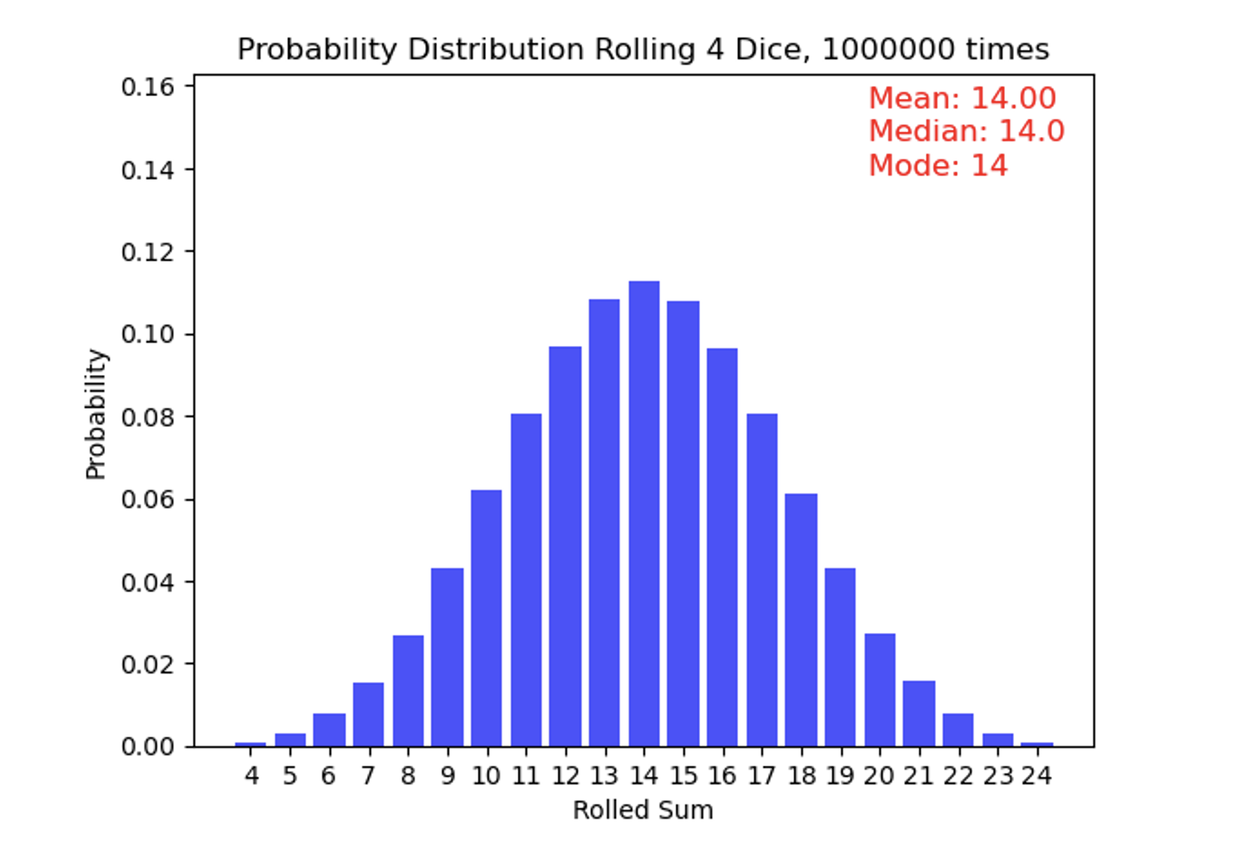
Now we roll 4 weighted dice one million times and add up what their faces show. These dice have small pieces of metal inside of them so that low numbers come up more often than high numbers. This results in a skewed distribution where combinations of lower numbers happen more frequently than higher numbers. This is an example of a positively skewed distribution, since the “tail” is longer on the right-hand side of the measures of central tendency. Also note that the mean is greater than the median, which is greater than the mode.