Lesson 3: Statistical Models
Front page
Nonlinear weather phenomena

Nonlinear weather phenomena.
The image displays a rectangular chalkboard with a dark brown frame and a chalk tray at the bottom, including a small white piece of chalk and an eraser. The left half features text explaining non-linear equations in a yellow font. A graphical representation of the Lorenz attractor is on the right side, showing a complex set of interwoven loops in pale yellow against a black background. The loops resemble butterfly wings, contained within a coordinate grid.
Planes zipping through the air

Planes zipping through the air.
The image shows an aircraft flying low over a grassy field, with air spiraling into a dramatic vortex in its wake. Air movements are highlighted with red smoke. The plane is seen from behind, with its propeller and wings visible. The vortex forms a distinct spiral pattern, swirling through the sky with a vivid mix of red and shades of gray. In the background, there is a line of dark green trees under a bright blue sky. The colors are striking, with the red smoke contrasting sharply against the blue sky.
Cartoon linking the butterfly effect to weather

Cartoon linking the butterfly effect to weather.
This is a black-and-white four-panel comic strip from "Zits" by Jerry Scott and Jim Borgman. In the first panel, two characters are standing outside. The one on the left is speaking, saying they have been reading about chaos theory. The other character, standing to the right, responds with "Yeah?" In the second panel, the character on the left explains that chaos theory claims a butterfly flapping its wings could cause a storm on the other side of the world. The other character replies with "Huh." The third panel shows a butterfly in a circular frame, emitting a loud "BURRP!" sound. The final panel shows the two characters sitting outside during a violent storm. One character asks, "Do you believe it?" The other responds with "Seems unlikely."
Statistical models: Why and How?
ECMWF forecast of 2-meter temperatures

ECMWF forecast of 2-meter temperatures.
This image is a color-coded weather map of the United States illustrating the 2-meter AGL (Above Ground Level) temperature forecast in degrees Fahrenheit. The map is divided by state boundaries and displays temperatures ranging from below 10°F in the northwest to above 70°F in the southeast. The northwestern region, including parts of the Rocky Mountains and Pacific Northwest, is colored in purples and blues indicating cold temperatures from around 4°F to 20°F. Moving eastwards, the Midwest and Great Plains show a blend of blues and greens, representing temperatures between 20°F and 40°F. The southeastern United States, particularly along the Gulf Coast, is depicted in shades of red and orange, showing warmer temperatures from 60°F to 75°F. The map includes informational text about its source and date, with temperature values numerically labeled across different regions.
Map of the sites for GFS MOS

Map of the sites for GFS MOS.
The image is a map of the United States divided into geographic regions, each represented by differently colored dots. The main map covers the contiguous United States, while additional insets show Alaska and Hawaii. Colors vary by region: red represents the west coast, purple covers the interior west, green spans the upper Midwest, blue is in the central and south-central areas, yellow covers the southeast, and orange is in the northeast. Each dot represents a specific GFS MOS location within those regions. Both Alaska and Hawaii follow similar color schemes, with Alaska showing purple and blue, and Hawaii in red. State boundaries are outlined in black, providing clear demarcations.
MOS Tables
Both 44 degrees Fahrenheit (GFS MOS table for KHOU)

Both 44 degrees Fahrenheit (GFS MOS table for KHOU).
The image displays a grid layout of GFS MOS data, titled "KHOU GFS MOS GUIDANCE," dated February 2, 2022, at 1800 UTC. The grid is organized into columns and rows, featuring various weather variables and corresponding numerical values. Weather variables include HR, N/X, TMP, DPT, and others, with numbers below each representing different data points. Notably, the "TMP" row has the numbers 44 highlighted in red boxes. The values are systematically aligned and spaced, offering a structured display of information.
Temperatures declining through much of the period (GFS MOS table for KHOU)

Temperatures declining through much of the period (GFS MOS table for KHOU).
The image displays a detailed GFS MOS table for KHOU, formatted in a grid. It shows various columns representing different weather parameters over time, with specific metrics for each parameter. The columns are labeled at the top with dates and times. The data is arranged in rows with parameters like HR, TMP, DPT, CLD, and others. Numbers fill most cells in uniform spacing. A section in the middle has a yellow background highlighting declining temperature values.
Maximum temperature forecast was actually 63 degrees Fahrenheit (GFS MOS table for KHOU)

Maximum temperature forecast was actually 63 degrees Fahrenheit (GFS MOS table for KHOU).
The image displays a GFS MOS data table, specifically for the location labeled "KHOU." The table is organized into rows and columns with various headings. The top row includes the identifiers "GFS MOS GUIDANCE" and the date "2/02/2022," followed by a time "1800 UTC." Beneath these headings are multiple categories such as HR, TMP, DPT, CLD, WSP, P06, etc., each filled with corresponding numerical data. The data is structured in chronological order for specific intervals, detailing information that may include temperature, cloud cover, wind speed, precipitation, and other meteorological variables. A red box highlights a specific section, focusing on data from the 3rd and 4th of February showing that the maximum temperature for that period occurred at 06Z February 3. The numbers within offer specific measurements and codes related to weather conditions.
Minimum temperature forecast was 32 degrees Fahrenheit (GFS MOS table for KHOU)

Minimum temperature forecast was 32 degrees Fahrenheit (GFS MOS table for KHOU).
The image is a GFS MOS table for KHOU, with specific forecasts made at different hours across two days in February 2022. The table is outlined with rows and columns, labeled with headers at the top. The top row includes specific headers such as "HR," "N/X," "TMP," "DPT," and more, indicating different types of data, like temperature and wind. Below the header row, there are numerical data entries listed under each hour of the day in a series of columns. The rows include headers like "TMP" and "CLD," with corresponding numerical or coded data beneath. A column labeled "DT /FEB" indicates specific dates, and "1800 UTC" suggests the time reference. Some areas have highlighted backgrounds, like the number 32 at the intersection of the "TMP" row and "21" hours, showing the minimum temperature for the highlighted period.
Strong cold front passing through Houston around 06Z on February 3

Strong cold front passing through Houston around 06Z on February 3.
The image is a surface analysis weather map of the United States, detailing atmospheric conditions for February 3, 2022. It features numerous isobars, represented by curved red lines, with numerical values indicating pressure levels across the map. High and low-pressure systems are marked with blue "H" and red "L" symbols, respectively. Areas of precipitation are highlighted with various weather symbols, including cold and warm fronts depicted in blue and red lines with corresponding triangular and half-circle markers. The text “Houston” is prominently marked near the Gulf Coast region, with a cold front having just passed through. The map includes geographical outlines of U.S. states, labeled pressure and temperature readings, and various local weather markers depicted by numbers, letters, and symbols.
The highest MOS wind speed listed is 22 knots at 03Z on February 4 (GFS MOS table for KHOU)

The highest MOS wind speed listed is 22 knots at 03Z on February 4 (GFS MOS table for KHOU).
The image is a computer-generated table of GFS MOS data, specifically focusing on short-term weather forecasts. The top row indicates the data point, with "KHOU" likely representing a weather station or location code, and "GFS MOS GUIDANCE" referring to the weather model. The table provides data for different dates, marked as "2/02/2022," with time indicated as "1800 UTC." Columns represent different hours on two consecutive days, depicted as "3" and "4," signifying the third and fourth of February. Rows include various weather-related parameters, labeled with abbreviations such as "HR," "N/X," "TMP," "DPT," "CLD," and "WSP." Each row contains numerical data representing forecasts for the corresponding hour and date. Specific sections in the table, such as "WSP," are highlighted with a yellow background, with the maximum value "22" marked with a black rectangle.
A probability of 92 percent (GFS MOS table for KHOU)

A probability of 92 percent (GFS MOS table for KHOU).
The image displays a table filled with GFS MOS data for KHOU, organized under the header "GFS MOS GUIDANCE" with a timestamp of "2/02/2022 1800 UTC". The table contains multiple rows and columns, including labels such as HR, N/X, TMP, DPT, CLD, WSP, WDR, P06, and more. Each row and column are filled with numbers that likely represent meteorological values. One cell in the "P06" row is highlighted yellow with the number "92" in it, highlighting the probability of precipitation from 06Z to 12Z on February 3. The overall layout is structured with columns representing different time frames and rows indicating various weather parameters.
Appropriate 6-hour ranges (GFS MOS table for KHOU)

Appropriate 6-hour ranges (GFS MOS table for KHOU).
The image displays a tabular GFS MOS chart labeled "GFS MOS GUIDANCE" with date, location, and time headings at the top. The table columns are divided by date and hour, and rows list various weather data metrics coded with abbreviations, such as "TMP" for temperature, "WSP" for wind speed, and "CLD" for cloud cover. Numerical values and letters fill the table, likely representing forecasted weather conditions over different hours and days. One row labeled "Q06" has numbers enclosed in a red box, indicating a specific focus or highlight on these figures, which are the sequential digits "3 1 1 1".
”2“ refers to the six-hours from 00Z to 06Z (GFS MOS table for KHOU)

”2“ refers to the six-hours from 00Z to 06Z (GFS MOS table for KHOU).
The image is a detailed GFS MOS table for KHOU, providing guidance for February 3rd and 4th, 2022, at 1800 UTC. The table includes various weather parameters such as temperature, dew point, wind direction, and cloud coverage across different hours. The data is organized in columns representing specific times: 00, 03, 06, 09, 12, 15, 18, and 21 each day. A red box highlights specific columns with forecast information for February 3rd. Additionally, there is an annotation with an arrow pointing to a cell in the row labeled "P06," indicating a value of "2" that is shaded orange. This annotation also contains a text box at the left explaining, "This '2' covers the 00Z-06Z period."
MOS Temperature Forecasts
MOS Wind and Precipitation Forecasts
MOS and Climatological Extremes
06Z GFS MOS forecast

06Z GFS MOS forecast.
The image is a GFS MOS table from a weather forecasting model for Wilmington, labeled as "GFS MOS GUIDANCE." The data is dated 9/13/2018, at 0600 UTC. The table contains rows of weather variables labeled at the beginning of each line, such as TMP (temperature), CLD (cloud cover), and WSP (wind speed). Each column represents an hour and the table covers data for September 13-15. The WSP row, which indicates wind speed, is highlighted with a red rectangular box. The background of the table is light blue, with black numbers and letters forming the data.
METARS from 03Z, 06Z, 09Z, 12Z, 15Z, and 18Z

METARS from 03Z, 06Z, 09Z, 12Z, 15Z, and 18Z.
The image displays a sequence of METAR reports, formatted in rows and columns. Each row begins with an identifier, "KILM," followed by a series of numerical and alphanumeric codes that indicate specific weather conditions, times, and other atmospheric data. Notable elements include wind speeds and directions, cloud cover, temperature, and additional meteorological observations. The data are separated by spaces and appear in a monospaced font, giving it a structured and aligned appearance. One column is highlighted in red, emphasizing specific wind information such as "33034G46KT" and similar codes in subsequent rows.
Radar loop of Florence's landfall
Transcript of the Radar loop of Florence's landfall
The image is a radar loop showing Hurricane Florence's landfall near Wilmington, North Carolina, as observed by NEXRAD Level-II. The map is filled with swirling patterns of colors that indicate different levels of precipitation and reflectivity. At the center, near Wilmington, there is an intense red and orange area, representing high precipitation concentration. Surrounding this are bands of yellow, green, and blue, indicating varying levels of rainfall intensity, with blue areas showing lighter rain. The legend on the right-hand side of the image shows a color scale ranging from purple to red, with corresponding dBZ values from -25 to 75, signifying different precipitation intensities measured in decibels of Z (dBZ). The image is timestamped 09/14/2018 12:47:25 Z.
Ensemble model forecasts showing Florence slightly weakening

Ensemble model forecasts showing Florence slightly weakening.
The image is a graph depicting the early-cycle intensity guidance for Hurricane Florence (AL06) as of 0600 UTC on September 13, 2018. The graph plots forecast intensity (in knots) on the vertical axis against forecast period (in hours) on the horizontal axis. The forecast period spans from 0 to 132 hours, and the intensity ranges from 0 to 120 knots. Multiple colored lines, each labeled with different model acronyms, represent various intensity forecasts. The graph background is shaded in bands indicating different storm categories: tropical storm, and Categories 1 to 3 hurricanes. Most models predict a decrease in intensity over time, with initial intensities ranging from about 80 to 100 knots, dipping as the forecast period progresses. Model lines cluster initially but diverge significantly after 48 hours.
LAMP Guidance
LAMP update schedule

LAMP update schedule.
The image displays a blue background with the title "LAMP updates the GFS MOS" at the top in white text. Below, there are four green rectangular blocks labeled "1800 UTC MOS," "0000 UTC MOS," "0600 UTC MOS," and "1200 UTC MOS." Beneath each green block is a column of three-dimensional blue rectangles labeled with different UTC times for LAMP updates, ranging from 0000 UTC to 2300 UTC. To the right is a white speech bubble that says, "The following LAMP cycles update the 1200 UTC GFS MOS cycle."
Hourly predictions (LAMP for KUNV)

Hourly predictions (LAMP for KUNV).
The image displays a table of LAMP forecasts for "UNIVERSITY PARK" under the label "KUNV GFS LAMP 1530 UTC 5/19/2022". The table is organized with columns representing hours in UTC ranging from 16 to 16 of the next day, emphasizing a 24-hour period. Each row provides different weather parameters including temperature (TMP), dew point (DPT), wind direction (WDR), and more, with numerical or coded entries. The parameters are listed on the leftmost column. To the right, under the heading "Hourly forecasts", each cell contains data corresponding to a specific hour and weather parameter. A red mark highlights the words "Hourly forecasts".
Regional surface observations

Regional surface observations.
The image is a detailed weather map showing various meteorological data points across a geographic region near Lake Michigan. It displays numerous weather stations with data such as temperature, wind speed, and direction. The map is overlaid with a pale green grid indicating different town or city areas. Each station is marked by a small circle, with wind barbs indicating wind direction and speed. Temperatures are noted close to each circle, and some also have colored markers indicating flight categories based on visibility and weather conditions. Several stations color coded in red have low ceilings -- less than 1,000 feet. In the top right corner, there is a segment of Lake Michigan with blue shading. A scale bar shows distances in kilometers and miles. At the bottom, symbols and abbreviations explain the map data, such as wind speed and flight category codes.
Case Study: Model Changes and MOS Impacts
Grids
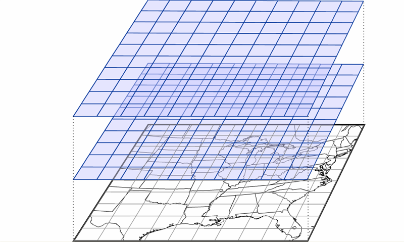
Grids.
The image displays three layered grids, each slightly tilted and overlaying one another, above a detailed map. The grids are represented by transparent blue lines forming square patterns, with the uppermost grid being the largest. Below, the black-and-white map shows geographical features and outlines of the eastern United States, including states and coastlines. The grid overlays suggest a method of mapping or data representation over the geographic map.
The National Blend of Models
List for version 4.1 of the NBM
| Model Name | Agency | Resolution | Cycles/Day | Members | Cycles Updated |
|---|---|---|---|---|---|
| ACCESS-G | BoM Australia | 12 km | 2x | 1 | 07, 19 |
| ACCESS-GE * | BoM Australia | 35 km | 4x | 18 | 02, 08, 14, 20 |
| EC MOSD | ECMWF | N/A (Stations only) | 2x | 1 | 08, 20 |
| EC MOSE | ECMWF | N/A (Stations only) | 2x | 50 | 09, 21 |
| ECMWFD | ECMWF | 25 km | 2x | 1 | 08, 20 |
| ECMWFE | ECMWF | 50 km | 2x | 50 | 09, 21 |
| GDPS | CMC Canada | 25 km | 2x | 1 | 05, 17 |
| GEPS | CMC Canada | 50 km | 2x | 20 | 07, 19 |
| GEFS | NCEP | 25 km | 4x | 30 | 01, 07, 13, 19 |
| GFS | NCEP | 13 km | 4x | 1 | 05, 11, 17, 23 |
| GFS MOS STN | NCEP | N/A (Stations only) | 4x | 1 | 00, 06, 12, 18 |
| GLMP | NCEP | 2.5 km | 24x | 1 | Every hour |
| GMOS | NCEP | 2.5 km | 2x | 1 | 07, 19 |
| HiResW ARW | NCEP | 3 km | 2x | 2 | 04, 16 |
| HiResW ARW MEM2 | NCEP | 3 km | 2x | 1 | 04, 16 |
| HiResW FV3 | NCEP | 3 km | 2x | 1 | 04, 16 |
| HMON | NCEP | 1.5 km | 4x | 1 | 00, 06, 12, 18 |
| HREF | NCEP | 5 km | 2x | 8 | 07, 19 |
| HRRR | NCEP | 3 km | 24x | 1 | Every hour |
| HRRR-EXT | NCEP | 3 km | 4x | 1 | 03, 09, 15, 21 |
| HWRF | NCEP | 1.5 km | 4x | 1 | 00, 06, 12, 18 |
| LAMPMOS | NCEP | N/A (Stations only) | 24x | 1 | Every hour |
| MELD | NCEP | 2.5 km | 24x | 1 | Every hour |
| MMEBC | NCEP/WPC | 5 km | 4x | 1 | 00, 06, 12, 18 |
| NAM | NCEP | 12 km | 4x | 1 | 03, 09, 15, 21 |
| NAMMOS | NCEP | N/A (Stations only) | 4x | 1 | 03, 09, 15, 21 |
| NAMNest | NCEP | 3 km | 4x | 1 | 03, 09, 15, 21 |
| NAVGEMD | FNMOC | 50 km | 4x | 1 | 07, 19 |
| NAVGEME | FNMOC | 50 km | 2x | 20 | 06, 18 |
| RAP | NCEP | 13 km | 24x | 1 | Every hour |
| RAP-EXT | NCEP | 13 km | 4x | 1 | 00, 06, 12, 18 |
| RDPS | CMC Canada | 10 km | 4x | 1 | 04, 10, 16, 22 |
| REPS | CMC Canada | 15 km | 2x | 20 | 07, 19 |
| RTMA | NCEP | 2.5 km | 24x | 1 | Every hour |
| QMD | MDL | 2.5 km | 4x | 1 | 01, 07, 13, 19 |
| SREF | NCEP | 16 km | 4x | 24 | 01, 07, 13, 19 |
| REWPS * | CMC Canada | 2.5 km | 2x | 20 | 05, 17 |
| GEPS Waves | CMC Canada | 25 km | 2x | 20 | 07, 19 |
| NAVGEMD Waves | FNMOC | 100 km | 2x | 1 | 07, 19 |
| NAVGEME Waves | FNMOC | 50 km | 2x | 20 | 07, 19 |
| GFS WW3D Waves | NCEP | 25 km | 4x | 1 | 05, 11, 17, 23 |
| GEFS WW3E Waves | NCEP | 25 km | 4x | 30 | 01, 07, 13, 19 |
| WW3D HIRES Waves | NCEP | 9-17 km | 4x | 1 | 05, 11, 17, 23 |
| GLWU Waves | NCEP | 2.5 km | 4x | 1 | 02, 08, 14, 20 |
KHOU NBM Table — Standard deviations of temperature forecasts ("TSD")

KHOU NBM Table — Standard deviations of temperature forecasts ("TSD").
The image is a forecast table from the NBM with various meteorological readings listed in columns and rows. The table header includes station information, version details, and timestamps, displayed at the top in a horizontal format. The rows contain abbreviations such as TMP, DPT, and SKY, each followed by numerical data indicating measurements or forecasts. The numbers are organized in a grid, where each column represents a specific time or date, as indicated at the top of the table. The layout is dense, with little spacing between data points, and some temperature standard deviations are highlighted or bolded for emphasis.
Bias Correcting the NBM
Map of Nevada surface observation sites

Map of Nevada surface observation sites.
The image is a topographic map highlighting the state of Nevada and surrounding areas. The map is populated with numerous black circles interconnected by black lines, indicating weather stations across the region. There are clusters of circles around major cities such as Las Vegas and near the California border. Two prominent mountains are labeled: "White Mountain Peak 4342m" in California and "Wheeler Peak 3982m" in eastern Nevada. The map features labeled cities like Fresno and Bakersfield, providing geographical context.
Low clouds (on visible satellite imagery)

Low clouds (on visible satellite imagery).
The image is a satellite view of the United States, displaying the country's topography and weather patterns. The western part of the image shows the arid, brown terrain of the American Southwest, extending up to the greener and forested Pacific Northwest. A large swirling weather system dominates the central region, with dense white clouds indicating a cyclonic formation, most prominent over the Midwestern states. The eastern states are covered with a more dispersed cloud cover, extending over the Atlantic Ocean. Clear demarcations of the geographic regions, states, and mountain ranges are visible. The Gulf of Mexico is at the bottom right, bordered by a line of clouds.
Tennessee River Valley

Tennessee River Valley.
The image is a map showcasing a region in the southeastern United States. It highlights the Tennessee Valley, with a light yellow shaded area indicating the Tennessee Valley watershed. The map outlines state boundaries in black, covering parts of several states, including Kentucky, Tennessee, Alabama, Mississippi, and North Carolina. The Tennessee River is prominently depicted in blue, meandering through the highlighted area from the upper left to the lower center of the map. The surrounding regions are marked in a paler color to contrast the highlighted watershed area. County lines within the states are also visible, providing a detailed geographical division.
NBM run from 23Z on May 14, 2018

NBM run from 23Z on May 14, 2018.
The image is a detailed heat map of a region represented in various shades of red and orange, indicating temperature levels. The map includes several numbers scattered throughout, representing specific temperature values in degrees Fahrenheit. The colors range from deep red, signifying higher temperatures (in the mid-90s), to lighter orange and yellow, indicating slightly cooler areas (in the 80s). Blue lines traverse the map, representing rivers or other water bodies. The map is divided by state borders, marked in white. At the top edge of the map, there is a color scale bar ranging from shades of purple to red, corresponding to temperatures from 56 to 94 degrees Fahrenheit. A small black rectangle near the center-right section highlights a spot where the temperature is noted as 96 degrees. The bottom right corner of the image is marked with "Mon 23Z 14-May-18," indicating the date and time.