Lesson 6 Images
Lesson 6: Forecasting Precipitation: Controllers and Strategies
Forecasting Precipitation: Controllers and Strategies
Corresponding threat scores for 66-72 hour forecasts

Corresponding threat scores for 66-72 hour forecasts.
The image is a bar graph comparing the threat scores of different forecasting models over a 72-hour forecast period from November 2021 to November 2022. The title at the top reads ".25'' WPC -vs- NWP Guidance Threat 66-72 Hour Forecast". The y-axis is labeled "Threat Score" and ranges from 0.00 to 0.50 in increments of 0.05. The x-axis represents different months, spaced out in intervals, displaying Nov 21, Jan 22, Mar 22, May 22, Jul 22, Sep 22, and Nov 22. The graph includes four sets of colored bars per month: green for NAM, blue for GFS, pink for ECMWF, and red for WPC. Each bar represents the threat score for each model, with varying heights across the months, indicating changes in forecast accuracy. A legend at the bottom specifies which color corresponds to each forecasting model.
Map of estimated rainfall

Map of estimated rainfall.
The image is a color-coded weather map illustrating the observed precipitation over Ohio and surrounding areas for one day. The map displays various shades of blue, green, yellow, and red, indicating different precipitation levels, with dark blue representing lower amounts and red indicating higher amounts. Ohio is prominently featured, bordered by black lines, with surrounding states partially visible. The highest precipitation, marked in red, is concentrated near the northwest of the state. A color scale on the right shows measurements in inches, ranging from 0.01 to over 10. At the bottom left, a small NOAA logo is visible.
The Big Picture and Upward Motion
Strong warm advection

Strong warm advection.
The image is a weather map displaying temperature advection at the 850 mb pressure level over a large portion of the United States. The map features height contour lines drawn in black. These contours are irregularly shaped, indicating variations in geopotential height. Additionally, there are red and blue shaded areas signifying temperature advection at this pressure level, with red indicating warmer air advection and blue indicating cooler air advection. Light red contour lines indicate temperature gradients. The background is a light beige color, and various numbers annotate the map, representing numerical weather data such as temperature and wind speed.
Surface warm front

Surface warm front
The image is a weather surface analysis map of the United States. It features various meteorological symbols depicting pressure systems, fronts, and isobars. Red and blue lines with semicircles and triangles indicate warm and cold fronts. High-pressure areas are marked with blue "H" letters, and low-pressure areas with red "L" letters. Isobars, shown as thin red lines, snake through the map, connecting areas of equal atmospheric pressure, with numeric labels indicating pressure values in millibars. States are etched on the map in bold black outlines. The map provides a detailed snapshot of weather conditions across the country on July 14, 2010, showing a warm front running through southern Minnesota among other features.
Tracking air parcels through shortwave troughs

Tracking air parcels through shortwave troughs.
The image illustrates a meteorological concept with black and red contour lines on a white background. The black lines represent a 500-mb wave pattern with peaks and troughs, while the red dashed lines overlay the black, showing the pattern of vorticity. Two areas are shaded: a green area near the trough on the left and a blue area on the right, indicating movement and changes in vorticity. A red "X" marks the vort max the center of the image. An animated air parcel follows along the height contours, illustrating changes to its rotation and size. Two text boxes provide explanations of vorticity changes: the left in green and the right in blue.
GFS forecast prog

GFS forecast prog.
The image is a weather map depicting 500 mb geopotential height and vorticity across a section of North America. The map features contour lines in brown and black, indicating height variations and temperatures. Yellow and red shaded areas represent regions of higher vorticity, particularly concentrated in the northeastern part of the map. There is a subtle vort max located over eastern Ohio of note. The contour lines are dense and curved, with numbers indicating height values such as 580, 584, and 588 dm. The map also includes a color bar on the left, ranging from yellow to dark red, corresponding to increasing vorticity values. This weather map is overlaid with geographic boundaries.
Four-quadrant conceptual model

Four-quadrant conceptual model.
The image depicts a map overlay consisting of several black curved lines, representing 300-mb heights, stretching horizontally across a section of the United States. There is a large blue-shaded elliptical area centered over the central part of the country, indicating a region of maximum winds (a jet streak). The map also features four sets of dashed ellipses: two red and two green. The red ellipses are labeled "Upper-level Convergence" and are placed on in the left-entrance and right-exit regions of the jet streak. The green ellipses are labeled "Upper-level Divergence" and are located in the right-entrance and left-exit regions.
Idealized schematic of confluence and diffluence

Idealized schematic of confluence and diffluence.
The image is a diagram divided into two columns titled "Streamlines" and "Wind Vectors." At the top, there is a heading "Confluence/Diffluence and Convergence/Divergence." The "Streamlines" column on the left displays two arrows labeled "Diffluence" diverging and two arrows labeled "Confluence" converging. The "Wind Vectors" column on the right illustrates different arrow arrangements, showing how sometimes diffluence can lead to mass divergence, but also sometimes to mass convergence. Similarly, confluence can sometimes lead to mass convergence, but also sometimes to mass divergence.
Case Study: Incorporating the Big Picture
grid interpolation from a regional model
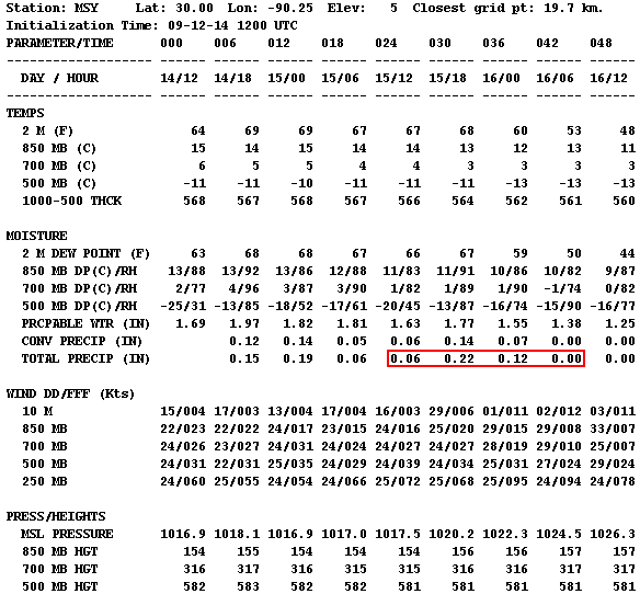
grid interpolation from a regional model.
The image displays a detailed meteorological data chart titled "Station: MSY" with the latitude, longitude, and elevation information. It covers various atmospheric measurements presented in tabular format. The chart lists parameters like "TEMPS," "MOISTURE," "WIND DD/FF (Kts)," and "PRESS/HEIGHTS," and breaks them down over specific times, denoted as "DAY / HOUR." The table includes temperatures at different altitudes, moisture levels, wind speeds and directions, and atmospheric pressures. Specific areas of the chart emphasize data in red, highlighting particular values related to total precipitation. The layout is organized with clear headers and columns, using a monospaced font for consistent alignment.
grid interpolation from a global model

grid interpolation from a global model
The image displays a detailed numerical weather data chart for a specific station indicated by "MSY" with latitude 30.00, longitude -90.25. The chart is presented in a plain text format, organized into rows and columns, each associated with specific meteorological parameters and times. The top rows display initialization time and are followed by columns representing forecast hours in intervals (e.g., 000, 006, 012, etc.). Parameters include temperature (in degrees Fahrenheit and Celsius), moisture levels, precipitation forecast (in inches), wind direction and speed (in knots), vertical velocity (in microbars per second), and other data like tropopause pressure and thickness. The chart uses space and alignment to organize the data, with temperatures, moisture readings, and other meteorological phenomena systematically listed under these intervals. Specific areas of the chart emphasize data in red, highlighting particular values related to total precipitation.
GFS forecast for 850-mb temperatures, winds, temperature advection, and frontogensis

GFS forecast for 850-mb temperatures, winds, temperature advection, and frontogensis.
The image is a weather map showing the southeastern United States with color-coded contours representing various meteorological data. Red lines depict temperature contours at the 850 hPa level, labeled in degrees Celsius. Shaded areas in blue and orange represent temperature advection, with blue indicating cold advection and orange indicating warm advection. Wind is indicated by wind barbs spread across the map, showing direction and speed. A purple star marks Greensboro, prominently labeled on the map in an area of warm advection. The image includes a color gradient on the right side, serving as a legend for the shading intensities.
09Z surface analysis

09Z surface analysis.
The image is a surface weather analysis map of the continental United States, dated March 18, 2021. It displays an array of meteorological symbols and contour lines in various colors representing different weather conditions. High-pressure areas are marked with blue "H" symbols, and low-pressure areas are denoted by red "L" symbols. Isobars are drawn in dark red. Blue lines with triangles indicate cold fronts, while red lines with semicircles represent warm fronts. Station models across the map show temperature, dewpoint, wind direction, and more. The map is dense with numerical data indicating temperature values in Fahrenheit, weather conditions, and atmospheric pressure readings. Various states across the map show varying temperatures and weather indicators.
GFS forecast for precipitable water valid at 06Z March 18

GFS forecast for precipitable water valid at 06Z March 18.
The image is a weather map displaying precipitable water in inches across the eastern United States. Shades of green, blue, and purple indicate different levels of moisture. Green hues dominate the northern region, covering states like Pennsylvania and New Jersey, indicating lower moisture levels, while blue shades spread across the central area, encompassing states like Tennessee and North Carolina, showing moderate moisture. In the southern part, near states like Louisiana, patches of purple suggest higher moisture content. The map contains black contour lines labeled with numbers indicating pressure levels in millibars, such as 1006 and 1018. State boundaries are clearly outlined, and the map includes a legend at the bottom showing a color scale from 0.25 to 3 inches.
Deep 500-mb trough over the Mississippi Valley

Deep 500-mb trough over the Mississippi Valley.
The image is a weather map showing the Geopotential Height, Cyclonic Vorticity, and Wind at the 500mb level across the United States. It is dated March 17, 2021, and projects data for March 18, 2021. The map uses a color scale ranging from yellow to red to indicate the intensity of cyclonic vorticity, with shades of red representing stronger vorticity. The map is covered in black contour lines showing Geopotential Height in decameters, with specific values like 552, 564, and 582 labeled across the map. Wind patterns are indicated by numerous wind barbs pointing in various directions. A significant area of cyclonic vorticity is centered over the central United States, marked by red and orange shades, particularly intense over Missouri and surrounding states. The background shows latitude and longitude lines.
09Z mesoanalysis of MUCAPE and lifted-parcel level

09Z mesoanalysis of MUCAPE and lifted-parcel level.
The image is a meteorological map of the United States, displaying a contour plot of weather data. Various colors and lines represent different meteorological values, specifically MUCAPE and lifted parcel levels. Yellow, green, and brown shading indicate lifted parcel levels, with numbers marked in black. Red contour lines with numbers indicate different values of MUCAPE. The map shows distinct overlays with denser data around the central and eastern United States, particularly over the Midwest and the Southeast. The map’s base features state boundaries outlined in thin brown lines.
0656Z radar image from KRAX

0656Z radar image from KRAX.
The image is a weather radar map centered on Raleigh-Durham, North Carolina, showing radar reflectivity. The map is overlaid with a network of highways and place labels. Bright colors, including green, yellow, and red, depict varying intensities of precipitation across the region, with green indicating lighter rainfall and red indicating heavier precipitation. The radar sweep is illustrated as a large, semi-circle expanding across the map, covering most of North Carolina and some surrounding states. Different shades of blue and green dominate the left and top portions, transitioning to yellow and red areas, indicating more intense weather activity. The map is marked with geographic and meteorological information, and colored scale bars indicate the reflectivity levels in decibels (dBZ) on the right side.
Full-sized image (Ensemble Plumes)

Full-sized image (Ensemble Plumes).
The image is a graph titled "NCEP SREF Plume for Total-QPF at GSO," showing quantitative precipitation forecasts. The graph has a white background with alternating light and dark gray vertical sections. Multiple colored lines represent different forecast models, showing the projected precipitation over time from March 17 to March 21. A red star labeled "0.53"" marks a point well above all of the lines at that time, indicating significant precipitation on March 18.
Getting Quantitative with Upward Motion
Upward-directed pressure gradient force balances the downward-directed force of gravity

Upward-directed pressure gradient force balances the downward-directed force of gravity
The image features a translucent blue cube centered between two arrows. The arrow above the cube is red, pointing upwards, labeled "Pressure Gradient Force." The arrow below the cube is purple, pointing downwards, labeled "Gravity." The arrows and labels suggest opposing forces acting on the cube. The background is white.
Model initialization for 700-mb heights and omega

Model initialization for 700-mb heights and omega
The image is a weather map depicting 700mb vertical velocity across parts of North America, with contour lines indicating geopotential heights. The map shows various colors ranging from light green to dark green, indicating different velocity values, overlaying a geographical outline of the continental United States. The contour lines are labeled with numbers like 3000, 2940, 2910, and 2680. Areas with positive values are highlighted and marked with text annotations. A prominent red arrow and circle emphasize regions of positive values, while another annotation highlights a negative sign in the units in the top-left corner. A color scale bar at the bottom provides a range of values from negative to positive.
The Flaws of Model QPF
Area Forecast Discussion

Area Forecast Discussion.
The image is a typed weather forecast report on a light gray background. The text is predominantly black with some phrases highlighted in red for emphasis. The forecast discusses weather conditions for Tuesday to Wednesday, including a shortwave ridge along the East Coast breaking down as a broad trough moves into the Ohio Valley. The report highlights potential precipitation but spuriously high model precipitable water forecasts. Certain weather models and their predictions are discussed, with attention to precipitation timing and temperature expectations in the mid-upper 80s Fahrenheit.
Transcribed Text:
TUE-WED...SHORTWAVE RIDGE ALONG THE EAST COAST WILL BREAK DOWN AS A BROAD TROUGH MOVES INTO THE OHIO VALLEY. SOUTHWESTERLY FLOW AHEAD OF THIS SYSTEM WILL CONTINUE TO ADVECT MOISTURE INTO THE AREA. FLOW SHOULD BE STRONG ENOUGH TO PREVENT ANY MESOSCALE INFLUENCE FROM THE EAST COAST SEA BREEZE. DESPITE THE DEEP MOISTURE...CATEGORICAL MAV POPS SEEM TOO HIGH AND MAY BE KEYING IN ON THE SPURIOUS 2.3+ INCH PWATS USING WARM SEASON EQUATIONS. NEVERTHELESS...SOME SITES WILL RECEIVE PRECIPITATION TOMORROW. BEST LARGER SCALE FORCING ALOFT ASSOCIATED WITH THE ENTRANCE REGION OF AN APPROACHING JET WILL ARRIVE LATE TUE NIGHT BUT WITH THE LOSS OF DAYTIME HEATING AND SUBSEQUENT INSTABILITY...WILL AGAIN FORECAST POPS BELOW THE MAVS. NAM-WRF TIMING SEEMS MOST REASONABLE GIVEN THE PREVIOUS FLIP-FLOPPING IN THE GFS. DRIER AIR SHOULD MOVE INTO THE NORTHERN ZONES WED MORNING BEHIND THE FRONT. FARTHER SOUTH...MOISTURE AND SCATTERED PRECIPITATION WILL LINGER INTO THE AFTERNOON. SLIGHTLY COOLER AIR WILL MOVE INTO THE AREA AS WELL...WITH HIGH TEMPERATURES IN THE MID-UPPER 80S.
Corresponding 23Z radar image

Corresponding 23Z radar image.
The image is a weather radar map showing precipitation patterns over the northeastern United States. A vertical line of intense storms stretches from the top to the bottom of the image, shown in bright colors ranging from green to red, indicating varying intensities of rainfall. The red areas suggest heavy rainfall, while green indicates lighter precipitation. Surrounding this main line, pockets of blue signify scattered, lighter showers. The map's background is black, with state boundaries outlined in a thin orange line.
CAM forecast from 12Z on August 9, 2020, valid at 18Z on August 10

CAM forecast from 12Z on August 9, 2020, valid at 18Z on August 10.
The image is a weather map depicting NAM 3km Near-Surface Reflectivity and 10m Wind in knots across the central United States. The map features a grid of thin black lines representing latitude and longitude. A red rectangle outlines a specific area covering parts of the Midwest, including Iowa and surrounding states. Green patches within this rectangle indicate areas of precipitation. Small black wind barbs evenly distributed across the map depict wind direction and speed. A color scale on the right side ranges from light green to bright purple, indicating reflectivity levels in dBZ. The title and relevant data, such as initialization time and forecast hour, are displayed at the top of the map.
18Z regional radar mosaic

18Z regional radar mosaic.
The image displays a weather radar map showing a large storm system over the central United States. The map indicates states with faint boundary lines, and a significant storm cluster is primarily centered over Iowa and Illinois. The storm system is depicted in various colors indicating intensity—green for lighter rain, yellow for moderate, and red for heavy precipitation. There are surrounding areas of scattered green patches indicating light rainfall. The western Great Lakes are visible in the upper-right corner. Yellow outlines emphasize the areas under a severe thunderstorm watch.
Navigating Model QPF
New Orleans, Louisiana

New Orleans, Louisiana.
The image is a map of the United States in a solid blue color. All states are depicted without visible borders or labels. A small red dot marks the location of New Orleans, Louisiana. A black and white text box next to the dot labels the city as "New Orleans, LA."
0.35 inches verified at KMSY

0.35 inches verified at KMSY.
The image is a screenshot displaying a series of METAR reports formatted in lines of text, each containing coded information. The text is arranged in a monospaced font across the image, with each line beginning with a sequence of letters and numbers. This sequence typically includes date-time markers, weather station identifiers, and various meteorological codes indicating weather conditions, temperatures, air pressure, and other related data fields. Precipitation totals are highlighted, summing to 0.35 inches. The background of the image is plain white, providing a stark contrast to the black text, making it easy to read. The codes appear dense and are uniformly spaced, extending horizontally from left to right.
Understanding Precipitation Climatology
Graph of daily normal and raw average high temperatures

Graph of daily normal and raw average high temperatures.
The image is a line graph showing the daily normal and raw average high temperatures in State College, Pennsylvania. The x-axis represents the date, ranging from January 1st to December 31st. The y-axis shows temperature in degrees Fahrenheit, ranging from 0°F to 90°F. Two lines are plotted: a blue line representing the 1991-2020 Raw Average and an orange line representing the 1991-2020 Official Normal. The blue line shows more variability with frequent fluctuations, while the orange line is smoother, providing a steady trend. The graph indicates a rise in temperatures from a low in January, peaking mid-year around July, and then descending back towards lower temperatures by December.
Plot of daily record maximum and record lowest maximum temperatures

Plot of daily record maximum and record lowest maximum temperatures.
The image is a graph representing the daily record maximum and lowest maximum temperatures in State College, Pennsylvania. The x-axis displays dates throughout the year, ranging from January 1st to December 31st. The y-axis indicates temperature in degrees Fahrenheit from -20°F to 120°F. Two curves are shown: one in red for record maximum temperatures and another in blue for record lowest maximum temperatures. The red curve hovers higher on the graph, peaking around July before descending, while the blue curve follows a similar pattern lower on the graph. Temperature points are marked as dots along the lines. A legend beneath the graph distinguishes the red and blue lines.
Eureka, California

Eureka, California.
The image is a line graph depicting daily mean maximum temperatures and extremes for Eureka, California (WSO CA). The vertical axis represents temperature in degrees Fahrenheit, ranging from 20 to 100. The horizontal axis denotes days of the year, marked from January to December. A red line shows daily temperature extremes, while a blue line indicates minimum extremes. A smooth black curve illustrates the mean maximum temperature over the year. The red line remains above the black line, and the blue line lies below it.
Pensacola, Florida

Pensacola, Florida.
The image is a map of the contiguous United States colored in solid blue. Each state boundary is outlined with thin black lines. A label with the text "Pensacola, FL" accompanied by a small black dot and a red marker is present at the western tip of Florida, near the Gulf of Mexico. The text is inside a white rectangle with a black border, pointing to the marker on the map.
Hurricane Opal

Hurricane Opal.
The image is a map illustrating the path of Hurricane Opal in 1995, depicted on a map of the eastern United States and parts of Mexico and the Caribbean. The trajectory begins in the Yucatán Peninsula, shown in light green, indicating a tropical depression. The path then turns yellow and red as it transitions into a tropical storm and hurricane over the Gulf of Mexico. The storm continued into major hurricane status shown in dark red. The path turns green as it travels inland, representing its weakening to a tropical depression through the central U.S. and finally moving northeast as an extratropical system marked with black crosses. The map has a beige background representing land and light blue for water. A legend in the top left explains the color and symbol coding. The text "Opal 1995" is positioned in the bottom right corner.
Forecasting Extreme Precipitation
Narrow swath of 6 - 8 inches of rain

Narrow swath of 6 - 8 inches of rain.
The image is a weather map depicting rainfall data for the northeastern United States. Various shades of green, yellow, orange, red, and blue indicate different rainfall totals, with green representing lighter rain and progressing to red for heavier rainfall. The map covers areas from Pennsylvania to Massachusetts, extending into the Atlantic Ocean. Key landmarks and city names are visible, like New York, Boston, and Philadelphia. Several purple circles with numeric values are scattered across the map, representing rainfall amounts in inches. Prominent numbers include 8.39 near northern New Jersey and 7.26 near Philadelphia. Overlapping this visual are two circular logos in the top left corner, one representing NOAA and the other for the National Weather Service.
12-hour QPF map from WPC

12-hour QPF map from WPC.
The image is a weather map of the contiguous United States displaying a 12-hour Quantitative Precipitation Forecast (QPF). Regions are color-coded based on expected precipitation levels, ranging from light green to dark red, indicating increasing amounts of rainfall. The heaviest precipitation, shown in dark red and purple, is concentrated in the northeastern states, particularly over New York and surrounding areas. Moderate levels of precipitation, in light to dark green, cover parts of the Midwest, South, and Western regions. The map features state boundaries and is predominantly covered in green shades. A NOAA logo is located in the bottom right corner.
Forecast issued the day before

Forecast issued the day before.
The image is a weather map of the United States depicting precipitation levels over a 12-hour period. The map features color gradients to represent varying precipitation amounts, ranging from light green to dark red, indicating an increase in rainfall. The heaviest precipitation, shown in red, is concentrated over the northeastern part of the United States, particularly around Pennsylvania and New York. Light green areas indicate lighter rain, covering parts of the Midwest and extending to the southern and southeast regions. The map includes state boundaries for reference and a color scale on the left side that quantifies precipitation levels from 0.01 to 20.00 inches. The bottom left corner contains text related to the forecast details. The NOAA logo is located in the bottom right corner of the map.
03Z run on September 1

03Z run on September 1
The image is a weather forecast graph from NOAA's Storm Prediction Center's Plume Viewer Version 2.0. It displays a series of color-coded lines representing different forecast models for total precipitation (Total-QPF) at LGA from September 1st, 2021. The graph’s x-axis shows time with labels starting from 06z on September 1st to 18z on September 4th, divided into sections by day. The y-axis measures precipitation in inches, ranging from 0 to 6.0. The lines, in various colors like pink, orange, yellow, and blue, depict different model runs, with each line showing forecast outcomes over the specified timeframe. On the right side, there’s a legend identifying each colored line as a specific model member.
NBM predicted less than 2.5 inches of rain

NBM predicted less than 2.5 inches of rain.
The image displays three tables containing meteorological data for three locations: KNYC, KLGA, and KEWR. Each table lists data with headings such as DT, UTC, FHR, TXN, XND, TMP, TSD, DPT, DSP, SKY, SSD, WDR, WSP, WSB, GST, DSD, P06, Q06, Q12, DUR, T03, T06, T12, PZR, PSN, and PPL across different date and time segments: September 1, September 2, and September 3 of 2021. Each table comprises rows and columns filled with numerical data, separated primarily by spaces. The numbers 229, 230, and 202, within the red rectangles, are highlighted prominently, one in each table, standing out against the otherwise plain text. These numbers represent 6-hour precipitation forecasts in hundredths of an inch. The top-left corner of each table contains a label indicating its respective location and version information regarding the NBM V4.0 NBS Guidance, dated 9/01/2021 at 0000 UTC.
Major and dangerous rain event was on the way

Major and dangerous rain event was on the way.
The image is a weather map of the United States showing the Day 1 Excessive Rainfall Outlook. The map highlights different regions with varying risks of excessive rainfall using colored areas. The eastern United States, particularly the northeastern region, is marked with red and pink, indicating high to moderate risk levels. The southern part of Florida and areas in the Western United States, notably around Nevada and Utah, have yellow and green shaded regions, indicating slight to marginal risk levels. The map has a legend explaining that pink signifies 50% risk and above, yellow signifies 10-20% risk, and green signifies 5-10% risk. The map includes state borders and the NOAA logo in the bottom left corner.
Atmospheric Rivers
Example from January 31, 2024

Example from January 31, 2024
The image is a map showing total precipitable water across the North Pacific Ocean, with a focus on the United States and Mexico. A gradient of colors is used to represent varying levels of precipitable water, ranging from deep purple indicating lower levels to orange suggesting higher levels. The map displays latitude and longitude markers with labels for lines of 10-degree intervals. A black contour line is used to show the path of a moisture flow from around 10°N, 170°W towards the west coast of the United States. The map's top left corner includes a logo with the text "CIMSS." A scale bar on the right translates color intensities into precipitable water values in inches and millimeters. The top of the image has the label "Total Precipitable Water 2024-01-31 2100 UTC."
Scale spans five categories from weak to exceptional

Scale spans five categories from weak to exceptional.
The image is a chart depicting the categorization of atmospheric rivers (AR) based on their duration and maximum Integrated Vapor Transport (IVT) magnitude. The chart is a grid with categories labeled from bottom to top as "Not an AR," "Weak," "Moderate," "Strong," "Extreme," and "Exceptional." The AR Duration is on the horizontal axis, ranging from 0 to 72 hours, while the Maximum IVT magnitude, measured in kg m-1 s-1, is on the vertical axis, ranging from 0 to 1,250. Each category is color-coded: "Not an AR" is gray or white, "Category 1" is light blue, "Category 2" is green, "Category 3" is yellow, "Category 4" is orange, and "Category 5" is red. A legend on the right correlates these categories, ranging from Cat 1 to Cat 5, with descriptions of the levels of hazard and benefits. Cat 1 is primarily beneficial (light blue), and Cat 5 is primarily hazardous (red).
Persistent orographic lift

Persistent orographic lift.
The image illustrates the concept of atmospheric rivers using a computer-generated graphic. It prominently features a blue, ribbon-like band representing an atmospheric river, flowing from the ocean over a mountainous landmass labeled "California." The band is depicted as carrying condensed water vapor, shown as raindrops and snowflakes falling over the mountains. An arrow labeled "Water Vapor Cools" points downward, indicating the cooling effect of the vapor as it moves inland. The background includes a map-like depiction of the land and ocean in natural tones of green and brown. The image is overlaid with text explaining the significance and impact of atmospheric rivers, especially in the Western United States. At the bottom right, there is a NOAA (National Oceanic and Atmospheric Administration) logo. The image is not to scale.
Cascade Mountains

Cascade Mountains.
The image is a detailed topographic map of the Pacific Northwest region, covering parts of British Columbia, Washington, Oregon, and northern California. It highlights major mountain peaks and cities along the Cascade Range. The map is oriented with north at the top. The Cascade Range is marked prominently with mountain peaks such as Mount Baker, Mount Rainier, Mount St. Helens, Mount Adams, Mount Hood, the Three Sisters, Mount McLoughlin, and Mount Shasta, all with their elevations in feet indicated. Key cities shown include Vancouver, Seattle, Portland, and Bend, among others. Major rivers, such as the Columbia River, are visible and labeled. The map features a mix of blues, greens, and browns to depict various natural features like water bodies, vegetation, and elevation changes.
2-10 inches of liquid throughout the Cascades and coastal mountain ranges

2-10 inches of liquid throughout the Cascades and coastal mountain ranges.
The image is a detailed map showing observed 24-hour precipitation levels across the Pacific Northwest, specifically in parts of Washington state and northern Oregon. It is dated as valid at 12 AM PT on November 5th. Various colors and numbers are overlaid on the geographic map to indicate precipitation measurements, measured in inches. The values range from low (0 inches) to high (over 9 inches), with colors ranging from blue and green for lesser amounts to red and purple for the highest amounts. The background of the map shows geographical features including cities, rivers, and terrain. A color scale is present on the right-hand side of the map, ranging from gray for the lowest precipitation to purple for the highest. At the bottom left is a source citation: NOAA/NWS Western Region.
Map of power outages and damage photos from Washington

Map of power outages and damage photos from Washington.
The image is a collage of four sections. The first section displays a map of Washington with regions color-coded to indicate power outage severity. Blue represents 0% outage, yellow 10%, orange 30%, red 60%, and dark red 100%. The map shows major areas affected by the outages. Text on the left displays customer data: "Customers Tracked: 3,233,329," "Customers Out: 210,548," "Last Updated: 2022-11-04 10:39:31 PM".
The second section shows a photograph of a road with fallen trees and debris, labeled "US-2 near Skykomish, WA". The road is partially obscured by vegetation and large pieces of timber.
The third section features another road in Snohomish County, WA, with several damaged utility poles leaning over, wires hanging low, illuminated by car headlights against a dark, wooded background.
The fourth section shows a flooded dirt road in a forested area labeled "SR 410 near Greenwater, WA," with scattered debris, including logs and rocks. The area is wet, and traffic cones are visible in the background.
Map showing the proportion of National Flood Insurance Program insured losses due to atmospheric rivers

Map showing the proportion of National Flood Insurance Program insured losses due to atmospheric rivers.
The image is a map of the western United States with various percentages displayed over different locations. These percentages represent the percentage of insured losses due to Atmospheric Rivers (ARs) from 1987 to 2017. Red circles accompany each location-specific percentage. The map shows mountainous terrain and is overlaid with state boundary lines. On the right, bold white text reads: “Percentage of insured losses due to ARs (1987-2017).”
August 2, 2022 drought monitor

August 2, 2022 drought monitor.
The image is a drought map of California from the U.S. Drought Monitor, dated August 2, 2022. It highlights different drought conditions across the state using a color-coded system. The map shows sections of California classified into varying levels of drought severity: yellow for "Abnormally Dry", tan for "Moderate Drought", orange for "Severe Drought", red for "Extreme Drought," and dark red for "Exceptional Drought." The majority of the state is covered in shades of red and dark red, indicating significant drought. To the right of the map is a table detailing drought conditions over time, with categories for current, last week, three months ago, and one year ago. The percentages indicate changes in drought conditions as time progresses. Below the table are details such as the map's author, Curtis Riganti from the National Drought Mitigation Center, and logos from USDA, NDMC, and NOAA.
July 4, 2023 drought monitor

July 4, 2023 drought monitor.
The image is a map from the U.S. Drought Monitor, depicting drought conditions in California as of July 4, 2023. The map outlines California's boundaries, with regions shaded in various colors to indicate drought intensity levels. Yellow represents areas that are "Abnormally Dry" (D0), covering parts of the state's northwest and southeast regions. A tan color indicates areas of "Moderate Drought" (D1) in southwestern areas. Blue lines mark rivers and water bodies. To the right, a table details the percentages of the state experiencing different drought conditions over time. The document includes logos of the USDA, NDMC, and NOAA at the bottom.
Map of atmospheric river frequency

Map of atmospheric river frequency.
The image is a world map showing the average number of Atmospheric Rivers (ARs) per year along various coastlines. Highlighted regions are marked with colored circles: red for 16+ ARs, orange for 8+, and yellow for 4+. These circles are mainly concentrated along the North American west coast, parts of the North Atlantic, Europe, West Africa, Southeast Asia, and South America's western and southern coasts. The map uses a satellite imagery background to illustrate landmasses and oceans, with black lines denoting national boundaries.
12-hour GFS forecast for IVT values valid at 00Z on January 10

12-hour GFS forecast for IVT values valid at 00Z on January 10.
The image is a weather map of the United States illustrating integrated vapor transport, measured in kg/m/s, with data from the 0.25° GFS model. The map is overlaid with black contour lines indicating 700-hPa geopotential height values. A dense cluster of contour lines is centered over the Great Lakes region, suggesting a low-pressure system. Arrows indicating vapor transport direction and intensity are concentrated on the eastern U.S. coast, colored from yellow to purple, depicting increasing intensity from west to east. The color gradient at the bottom marks the scale ranging from 250 to 1600 kg/m/s. The western U.S. shows lighter colors and fewer arrows.
Moderate risk (level 3 out of 4) for flash flooding with a lead time of five days

Moderate risk (level 3 out of 4) for flash flooding with a lead time of five days.
The image is a weather map displaying a forecast of excessive rainfall risk for the northeastern region of the United States. The map highlights different risk levels using colored zones. The northeastern coast, covering parts of New England and the mid-Atlantic, is shaded in red, indicating a moderate risk (MDT) with at least a 40% probability of rainfall exceeding flash flood guidance. Surrounding the red area is an orange zone, representing a slight risk (SLGT) with at least a 15% chance. The green zone, labeled MRGL, indicates a marginal risk with at least a 5% likelihood. The text box at the top of the map states that this is the sixth time a moderate risk has been issued at Day 5 and the first time such a risk has been issued in the Northeast. A label at the bottom left corner identifies the forecaster as "SCHICHTEL" and notes the validity and issuance dates. The NOAA logo is included in the lower left.
Snow Forecasting Products and Problems
Kuchera Ratio versus maximum temperature in the air column up to 500 mb

Kuchera Ratio versus maximum temperature in the air column up to 500 mb.
The image is a line graph representing the Kuchera Snow-Liquid Ratio. The x-axis shows the maximum 1000-500 hPa temperature in degrees Celsius, ranging from -25 to 15, marked in increments of 5. The y-axis shows the snow to liquid ratio, ranging from -20 to 40 in increments of 10. A blue line with circular data points connects values from the coordinates (-25, 35) to (15, -21). The data points are labeled with their respective y-values: 35, 30, 25, 20, 15, 8, -1, -11, and -21. The plot is set on a grid for clarity and shows a general relationship of decreasing snow-liquid ratio with increasing maximum column temperature.
Larger images

Larger images.
The image shows two weather forecast maps side by side, depicting predicted snowfall for parts of the northeastern United States. The left map from TropicalTidbits.com illustrates total snowfall in inches, assuming a 10:1 snow-to-liquid ratio, with bright colors ranging from blue to pink and red, indicating varying snowfall depths. The scale on the right of the map shows an increment of colors corresponding to snowfall amounts. The right map from Weathernerds.org displays the total snowfall with dynamic ratio, using shades of blue and pink, with deeper colors indicating higher snowfall. Both maps highlight the northeastern states with detailed state boundaries and numeric snowfall estimations overlaying the regions.
Southern periphery of the predicted area of snow

Southern periphery of the predicted area of snow.
The image consists of two weather maps side by side, displaying total snowfall predictions for the northeastern United States. The left map, from TropicalTidbits.com, uses a color gradient ranging from blue to purple to indicate snow depth in inches, with darker shades representing higher amounts. The map shows snowfall predictions across areas including the Great Lakes region, New York, and New England, with a scale from 0 to over 24 inches. The right map, from Weathernerds.org, has a similar layout but uses different color gradients, focusing more on shades of blue to pink for varying snow amounts. It covers similar regions and uses a detailed scale present on the right side, which goes up to 35 inches. Both maps have black oval outlines highlighting a specific area across parts of Pennsylvania, Ohio, and New York that show vastly different predicted snowfall totals (produced by the same model forecast).
Larger images

Larger images.
The image consists of two weather maps side by side, displaying snow forecasts for parts of the northeastern United States and southeastern Canada. The left map shows "GFS Accumulated Positive Snow Depth Change (inches)" with areas colored in varying shades of pink, purple, and blue, indicating different snow depth changes. The right map presents "0.25° GFS Total Snow (in)" with similar color gradations representing total snowfall. Both maps include geographical outlines and latitudinal and longitudinal labels. Snow depths range from 0 to 48 inches, with a legend on each map indicating the scale of snowfall by color.
Differed greatly along the the southern periphery of the area of snow

Differed greatly along the the southern periphery of the area of snow.
The image is a side-by-side comparison of two weather forecast maps showing snow data for the northeastern United States and parts of Canada. The left map displays "GFS Accumulated Positive Snow Depth Change (inches)" with varying shades of pink, purple, and blue, indicating different snow depth changes. Darker colors represent greater changes, with the most intense shades indicating up to 18 inches. The right map shows "0.25° GFS Total Snow (in)" using similar color coding, where intense pinks and purples denote heavier snowfall amounts. Both maps feature geographic outlines and labels for reference. A black rectangle highlights a specific region across the northeastern United States, focusing on states such as New York and Pennsylvania where the forecasts differ greatly. Each map contains a color legend to interpret the snow data, situated on the right side of each map.
Total snow forecasts described earlier
Total snow forecasts described earlier.
The image shows two weather forecast maps side by side, depicting predicted snowfall for parts of the northeastern United States. The left map from TropicalTidbits.com illustrates total snowfall in inches, assuming a 10:1 snow-to-liquid ratio, with bright colors ranging from blue to pink and red, indicating varying snowfall depths. The scale on the right of the map shows an increment of colors corresponding to snowfall amounts. The right map from Weathernerds.org displays the total snowfall with dynamic ratio, using shades of blue and pink, with deeper colors indicating higher snowfall. Both maps highlight the northeastern states with detailed state boundaries and numeric snowfall estimations overlaying the regions.
Verification

Verification.
The image is a map titled "National Gridded Snowfall Analysis during 72h preceding 2023 February 25, 0:00 UTC." It depicts parts of the northeastern United States and southeastern Canada with various colors indicating snowfall depths. The map spans areas from Wisconsin and Michigan in the west to New England and the Mid-Atlantic states in the east. Snowfall is represented using a color gradient. Yellow and orange areas indicate higher snowfall, mostly in northern and northeastern areas, while blue shades represent lighter snowfall. Dark gray areas show regions where snowfall is not estimated. Two scales run along the right side: "Inches of depth" and "Elevation in feet." A small inset map at the top right shows the region's location in North America. The map includes geographical markers such as state lines, cities, and natural landmarks.
Freezing Drizzle and Freezing Rain
Annotated sounding

Annotated sounding.
The image depicts a meteorological skew-t log-P diagram, commonly used for displaying upper air soundings. The background features a grid with isotherms (slanted blue lines), isobars (horizontal blue lines), and mixing ratio lines (purple lines). Two thick black lines trace the temperature and dew point profiles corresponding to different pressure levels on the left vertical axis, measured in hPa, and altitude measured in meters. The right side of the image contains several annotations and numerical values. Notably, a shaded green area diagonal across the graph indicates a "Layer at or near saturation." Wind barbs, which represent wind speed and direction at various altitudes, appear vertically along the right side. The bottom displays a title with the date, “00Z 08 Mar 2023."
METARS between 02Z and 03Z on March 8 from Broken Bow, Nebraska

METARS between 02Z and 03Z on March 8 from Broken Bow, Nebraska
The image is a section of a weather report in text format, showcasing several rows of coded METAR data. The data is arranged in columns and rows, and each row begins with "KBBW," followed by numbers, letters, and various meteorological observations. Highlighted within the rows are instances of the text “-FZRA.” A prominent blue arrow points towards the string "I1002" in one of the rows, with a label in blue reading “1-hour ice accretion of 0.02” positioned at the tip of the arrow. The text is set against a plain white background.
Example from Dallas-Fort Worth, Texas from February 11, 2021

Example from Dallas-Fort Worth, Texas from February 11, 2021.
The image is a Skew-T log-P diagram, which is used to analyze atmospheric conditions. The diagram displays temperature (red line) and dew point (green line) profiles with altitude, marked in pressure levels on the vertical axis from 1000 mb at the bottom to 100 mb at the top. The grid is tilted, with temperature in Celsius marked horizontally. Wind barbs representing wind speed and direction are displayed on the right. A small inset in the top right corner shows a hodograph, illustrating wind speed and direction at different altitudes with curved lines. the -10ºC and 0ºC isotherms are highlighted in purple.
Predicted ice totals were nearly 50 percent lower

Predicted ice totals were nearly 50 percent lower.
The image is a side-by-side comparison of two weather forecast maps showing predicted ice accumulation over the northeastern United States. The map on the left is titled “Total Accumulated Freezing Rain QPF (in)” and the one on the right is labeled “Total Accumulated Ice (FRAM est.) (in).” Both maps cover the same geographic area, including states from the Midwest to New England.
Each map features color gradients ranging from light gray to dark red, indicating varying levels of ice accumulation, with specific measurements marked in inches. The maps use a color scale at the bottom, from 0.05 in light gray to 2 inches in dark red. Both maps show that the central region appears darker, indicating higher ice accumulation predictions.
Two blue arrows on the right map point to a region in New York, accompanied by text noting, “FRAM forecasts nearly 50% lower!” This suggests a significant difference in prediction values between the two maps for this area.