L3: Understanding Spatial Patterns
L3: Understanding Spatial PatternsThe links below provide an outline of the material for this lesson. Be sure to carefully read through the entire lesson before returning to Canvas to submit your assignments.
Lesson 3 Overview
Lesson 3 OverviewAs humans, we are predisposed to seeing patterns when there may not necessarily be any. This week, you will be using a mixture of qualitative and quantitative methods to examine the spatial distribution of crimes.

Text description of the examples of visualizations image.
This image provides examples of outputs from the analysis you will undertake in this lesson. It includes a boxplot separated by crime type, bar charts of crime over time, the output of a K-function analysis, a histogram, an interactive map of crime made with Leaflet, a mean center analysis output, and a kernel density estimate map.
Learning Outcomes
At the successful completion of Lesson 3, you should be able to:
- describe and provide examples of simple deterministic and stochastic spatial processes;
- list the two basic assumptions of the independent random process (i.e., no first or second order effects);
- outline the logic behind derivation of long run expected outcomes of the independent random process using the quadrat counts for a point pattern as an example;
- outline how the idea of a stochastic process might be applied to line, area and field objects.
- define point pattern analysis and list the conditions necessary for it to work well;
- explain how quadrat analysis of a point pattern is performed and distinguish between quadrat census and quadrat sampling methods;
- outline kernel density estimation and understand how it transforms point data into a field representation;
- describe distance-based measures of point patterns (mean nearest neighbor distance and the G, F and K functions);
- describe how the independent random process and expected values of point pattern measures are used to evaluate point patterns, and to make statistical statements about point patterns;
- explain how Monte Carlo methods are used when analytical results for spatial processes are difficult to derive mathematically;
- justify the stochastic process approach to spatial statistical analysis;
- discuss the merits of point pattern analysis and outline the issues involved in real world applications of these methods.
Checklist
Lesson 3 is one week in length. (See the Calendar in Canvas for specific due dates.) The following items must be completed by the end of the week. You may find it useful to print this page out first so that you can follow along with the directions.
| Step | Activity | Access/Directions |
|---|---|---|
| 1 | Work through Lesson 3 | You are in Lesson 3 online content now. Be sure to carefully read through the online lesson material. |
| 2 | Reading Assignment | Before we go any further, you need to read the chapter associated with this lesson from the course textbook:
This week you might find it helpful to read the relevant portions of the reading as you work through the exercises. The relevant pages of the reading are highlighted in the lesson commentary. Additionally, particularly this week, I suggest you take the quiz after working through the project activities. |
| 3 | Weekly Assignment | This week's project explores the spatial patterns of the St. Louis crime dataset you worked with in Lesson 2. Note that you will download new crime data from St. Louis for Lesson 3. PART A: Analyze spatial patterns through R functions |
| 4 | Term Project | There is no specific deliverable this week as the weekly assignment is quite involved. Be sure to get in touch with your peer review group to set a time to meet in Week 5. |
| 5 | Lesson 3 Deliverables |
|
Questions?
Please use the 'Discussion - Lesson 3' Forum to ask for clarification on any of these concepts and ideas. Hopefully, some of your classmates will be able to help with answering your questions, and I will also provide further commentary where appropriate.
Spatial Point Pattern Analysis
Spatial Point Pattern AnalysisIn classical spatial point pattern analysis, standard statistical concepts are applied to the description and assessment of spatial point patterns, using the concept of a spatial process. The essential idea is to compare observed patterns on maps (i.e., what we see in the world) to the patterns we expect based on some model of a spatial process. In this lesson, you will examine spatial patterns created using a variety of methods and then examine some real spatial data to better understand what processes might be driving different spatial patterns.
Fundamentals: Maps as Outcomes of Processes
Fundamentals: Maps as Outcomes of ProcessesRequired Reading:
Before we go any further, you need to read a portion of the chapter associated with this lesson from the course text:
- Chapter 8, "Point Patterns and Cluster Detection," pages 243 - 270.
Spatial analysis investigates the patterns that arise as a result of spatial processes, but we have not yet defined either of these key terms.
Here, the rather circular definition, "A spatial process is a description of how a spatial pattern might be generated" is offered. This emphasizes how closely interrelated the concepts of pattern and process are in spatial analysis. In spatial analysis, you don't get patterns without processes. This is not as odd a definition as it may sound. In fact, it's a fairly normal reaction when we see a pattern of some sort, to guess at the process that produced it.
A process can be equally well described in words or encapsulated in a computer simulation. The important point is that many processes have associated with them very distinct types of pattern. In classical spatial analysis, we make use of the connection between processes and patterns to ask the statistical question, "Could the observed (map) pattern have been generated by some hypothesized process (some process we are interested in)?"
Measuring event intensity and distance methods (section 8.3) and statistical tests of point patterns (section 8.4)
These sections are intended to show you that for at least one very simple process (a completely random process), it is possible to make some precise mathematical statements about the patterns we would expect to observe. This is especially important because human beings tend to have a predisposition to see non-random patterns, even if there is no pattern.
Don’t get bogged down with the mathematics involved. It is more important to grasp the general point here than the particulars of the mathematics. We postulate a general process, develop a mathematical description for it, and then use some probability theory to make predictions about the patterns that would be generated by that process.
In practice, we often use simulation models to ask whether a particular point pattern could have been generated by a random process. The independent random process (IRP), also described as complete spatial randomness (CSR), has two requirements:
- an event must have an equal likelihood of occurring in any location; and
- there must be no interactions between events.
The discussion of first- and second-order effects in patterns is straightforward. Perhaps not so obvious is this: complete spatial randomness (i.e., the independent random process) is a process that exhibits no first- or second-order effects. In terms of the point processes discussed above, there is no reason to expect any overall spatial trend in the density of point events (a first-order effect), nor is there any reason to expect local clustering of point events (a second-order effect). This follows directly from the definition of the process: events occur with equal probability anywhere (no trend), and they have no effect on one another (no interaction).
Stochastic processes in lines, areas, and fields
The basic concept of a random spatial process can be applied to other types of spatial object than points. In every case, the idea is the same. Lines (or areas or field values) are randomly generated with equal probability of occurring anywhere, and with no effect on one another. Importantly, the mathematics become much more complex as we consider lines and areas, simply because lines and areas are more complex things than points!
Do:
Now it is your turn to explore spatial processes. To do so, you will use R to generate a series of point patterns that are driven by different mathematical equations and methods that simulate first- and second-order processes.
Project 3, Part A: Understanding Random Spatial Processes
Project 3, Part A: Understanding Random Spatial ProcessesBackground
During the first part of this week's project, you will be examining randomness in the context of spatial processes. This is a critical issue, because human beings are predisposed to seeing patterns where there are none, and are also not good at understanding the implications of randomness.
For example, if you ask someone to think of a number between 1 and 10, in Western culture at least, there is a much better than 1 in 10 chance that the number will be a 7. Similarly, if data for the national or state lottery tells you that the numbers 3, 11, 19, 24, 47, and 54 haven't 'come up' for many weeks, that should not be your cue to go out and pick those numbers; yet, for some people, it is, out of a misguided notion that on average all the numbers should come up just as often as each other. This is true, but it has no bearing on which particular numbers should come up in any particular week.
It is our weakness at dealing with the notion of randomness on this basic level that makes gambling such a profitable activity for those who do understand, by which I mean the casino owners and bookmakers, not the gamblers... anyway... this week, the project is an attempt to develop your feel for randomness by experimenting with a random spatial pattern generator, or in other words, a spatial process.
Project 3, Part A has been broken down into three sections where you will be exploring the outcomes of different processes:
- the Independent Random Process;
- the Inhomogenous Poisson Process; and
- interactions between events.
Work through each section, and answer the questions that have been posed to help you construct your project 3A write-up.
Project Resources
For Part A of this lesson's project, you will need an install of RStudio with the spatstat package installed and loaded.
Summary of Project 3A Deliverables
For Project 3A, the items you are required to include in your write-up are:
- Screen shots showing the different point patterns you generated according to different random processes with accompanying commentary that explains the patterns were created. Specific questions have been included in each section to guide you with the type of commentary to include.
Project 3, Part A: The Independent Random Process
Project 3, Part A: The Independent Random ProcessThe independent random process, or complete spatial randomness, operates according to the following two criteria when applied to point patterns:
- events occur with equal probability anywhere; and
- the place of occurrence of an event is not affected by the occurrence of other events.
The spatstat package provides a number of functions that will generate patterns according to IRP/CSR. The 'standard' one is rpoispp, which is actually a Poisson point process. This does not guarantee the same number of events in every realization as it uses a background process intensity to probabilistically create events. An alternative is the spatial point process function runifpoint, which guarantees to generate the specified number of events.
Begin by making sure that the spatstat library is loaded into RStudio:
> library(spatstat)Then use the Poisson process to generate a point pattern. The rpoispp method takes one parameter, N, the number of events. N has been set to 100 in this case. Draw and examine the pattern in the Plots window.
> pp <- rpoispp(100)
> plot(pp)
After examining the pattern, use the up arrow key in the console, pressing it twice, to repeat the code that generates the pattern and then use the up arrow to repeat the line of code that draws the pattern. You should see the pattern change in the plots window. How similar or different is the second pattern?
It is often helpful to examine multiple realizations of a process to see whether the patterns exhibit any regularities. We can use R to generate and plot several realizations of the Poisson process at once so we can more easily compare them. The first line of code below sets a framework of three plots in one row for laying out multiple plots in the Plots window in RStudio. The subsequent lines generate the patterns and plot them.
> par(mfrow=c(1, 3))
> pp1 <- rpoispp(100)
> plot(pp1)
> pp2 <- rpoispp(100)
> plot(pp2)
> pp3 <- rpoispp(100)
> plot(pp3)
Deliverable
Now, using examples of patterns generated from the rpoispp() or the runifpoint() functions to illustrate the discussion, comment on the following topics/questions in your Project 3A write-up:
- Do all these IRP/CSR patterns appear 'random'? If not, how do they seem to differ from 'random' patterns? (Be sure to include example plots to help the reader understand your discussion points).
- Do some of the patterns exhibit 1st order effects? Or, conversely, 2nd order effects? Provide an example from your explorations, and explain how it is possible for such seemingly 'non-random' patterns to be generated by a completely random process.
Project 3, Part A: An Inhomogeneous Poisson Process
Project 3, Part A: An Inhomogeneous Poisson ProcessNow, you are going to look at the inhomogeneous Poisson process. This is a spatial point process that generates events based on an underlying intensity that varies from place to place. In other words, it departs from IRP due to a first-order trend across the study area.
To introduce a trend, we have to define a function in place of the fixed intensity value of the standard (homogenous) Poisson process.
> pp <- rpoispp(function(x,y) {100*x + 100*y})This tells R that the intensity of the Poisson point process varies with the x and y coordinates according to the function specified.
NOTE: if you want to visualize a 3D plot of any equation, you can simply copy and paste the equation into a Google search and an interactive 3D graph of the equation will appear. Google supports equation graphing through their calculator options.
You might also want to plot the density and the contours of points. The first line creates and plots a density plot. The second line overplots the points on top of the density plot. The pch parameter controls which graphical mark is used to plot the points. You can see a full list of different mark symbols here.
> plot(density(pp))
> plot(pp, pch = 1, add = TRUE)
To plot contours, use the following code:
> contour(density(pp))
> plot(pp, pch = 1, add = TRUE)
Make a few patterns with this process and have a look at them. Experiment with this by changing the x and y values (e.g.,: 100*x + 50*y) until you understand how they interact with one another.
We have also provided two additional functions for you to explore using this same procedure.
Vary the intensity with the square of x and y coordinates:
pp <- rpoispp (function(x,y) {100*x*x + 100*y*y})Vary the intensity with the distance from the center of the unit square:
pp <- rpoispp (function(x,y) {200*sqrt((x-0.5)^2 + (y-0.5)^2)})Deliverable
Now, using examples of patterns generated using rpoispp() with a functionally varying intensity to illustrate the discussion, comment on the following topics/questions in your Project 3A write-up:
- Do all these patterns appear random?
- How do they differ from the random patterns you generated in the previous section, if at all?
- Can you identify the presence of 1st order effects in each pattern through visual inspection?
Project 3, Part A: Processes with Interaction Between Events
Project 3, Part A: Processes with Interaction Between EventsFinally, we will introduce second-order interaction effects using one spatial process that can produce evenly spaced patterns (rSSI) and one that produces clustered patterns (rThomas).
Note that there are other available processes in the spatstat package in R (e.g., evenly-spaced patterns using rMaternI(), rMaternII() and clustered patterns using rMatClust() as well as rCauchy(), rVarGamma(), rNeymanScott(), rGaussPoisson()). You can feel free to experiment with those if you are interested to do so. You can find out about the parameters they require with a help command:
> help("rMaternI")rSSI is the Simple Sequential Inhibition process.
> pp <- rSSI(a, N) where a specifies the inhibition distance and N specifies the number of events.
Events are randomly located in the study area (which by default is a 1-by-1 square, with x and y coordinates each in the range 0 to 1), but, if an event is closer to an already existing event than the inhibition distance, it is discarded. This process continues until the required number of events (N) have been placed. As the inhibition distance is reduced, the resulting pattern is more like something that might be generated by IRP/CSR, although events are still not completely independent of one another.
rThomas is a clustering process.
> pp <- rThomas(a, b, N)a specifies the intensity of a homogeneous Poisson process (i.e., IRP/CSR), which produces cluster centers.
b specifies the size of clusters as the standard deviation of a normally distributed distance from each cluster center. This means that events are most likely to occur close to cluster centers, with around 95% falling within twice this distance of centers, and very few fall more than three times this distance from cluster centers.
N specifies the expected number of events in each cluster.
Experiment with at least these two models (rSSI and rThomas) to see how changing their parameter values changes the spatial pattern in the plots. In your experimentation, I suggest varying one parameter while keeping the other parameter(s) constant until you understand the parameter's behavior. Use the R commands we've already introduced in the earlier parts of this lesson in your explorations of the homogeneous and inhomogeneous Poisson processes to create graphics to illustrate your write-up.
Deliverable
Now, using examples of patterns that you generated by the rSSI() and rThomas() models to illustrate uniformity and clustered patterns, comment on the following topics/questions in your Project 3A write-up:
- Explain the basics of how each of the rSSI() and rThomas() models work.
- Do all the created patterns appear random?
- How do the patterns differ from the random patterns you generated in the first section, if at all?
- Discuss whether it is possible to visually identify that 2nd order effects are influencing the locations of events in these patterns.
Point Pattern Analysis
Point Pattern AnalysisWe saw how a spatial process can be described in mathematical terms so that the patterns that are produced can be predicted. We will now apply this knowledge while analyzing point patterns.
Point pattern analysis has become an extremely important application in recent years, not only because it has become increasingly easy to collect precise information about something (e.g., using GPS coordinates through mobile technologies) but also is extensively used in crime analysis, in epidemiology, and in facility location planning and management. Point pattern analysis also goes all the way back to the very beginning of spatial analysis in Dr. John Snow's work on the London cholera epidemic of 1854. In Part B of this week’s lesson, you will be applying a range of exploratory and spatial statistical methods that would have helped Dr. Snow identify the source of the cholera infection quickly and efficiently. See more information about Snow's contribution to epidemiology.
Where to start?
Where to start?Required Reading:
- Chapter 8, "Point Patterns and Cluster Detection," pages 247 - 260.
- Chapter 2.4, "Moving window/kernel methods", pages 28 - 30
Introduction to point patterns
It should be pointed out that the distinction between first- and second-order effects is a fine one. In fact, it is often scale-dependent, and often an analytical convenience, rather than a hard and fast distinction. This becomes particularly clear when you realize that an effect that is first-order at one scale may become second-order at a smaller scale (that is, when you 'zoom out').
The simplest example of this is when a (say) east-west steady rise in land elevation viewed at a regional scale is first-order, but zooming out to the continental scale, this trend becomes a more localized topographic feature. This is yet another example of the scale-dependence effects inherent in spatial analysis and noted in Lesson 1 (and to be revisited in Lesson 4).
A number of different methods can be used to analyze point data. These range from exploratory data analysis methods to quantitative statistical methods that take distance into consideration. A summary of these methods are provided in Table 3.1.
PPA Method | Points  Figure 3.2 Credit: Blanford, 2019 | Kernel Density Estimate  Figure 3.3 Credit: Blanford, 2019 | Quadrat Analysis  Figure 3.4 Credit: Blanford, 2019 | Nearest Neighbour Analysis  Figure 3.5 Credit: Blanford, 2019 | Ripley's K  Figure 3.6 Credit: Blanford, 2019 |
|---|---|---|---|---|---|
| Description | Exploratory Data Analysis Measuring geographic distributions Mean Center; Central/Median Center Standard Distance; Standard Deviation/Standard Deviational Ellipse | Exploratory Data Analysis Is an example of "exploratory spatial data analysis" (ESDA) that is used to "visually enhance" a point pattern by showing where features are concentrated. | Exploratory Data Analysis Measuring intensity based on density (or mean number of events) in a specified area. Calculate variance/mean ratio | Distance-based Analysis Measures spatial dependence based on the distances of points from one another. Calculates a nearest neighbor index based on the average distance from each feature to its nearest neighboring feature. | Distance-based Analysis Measures spatial dependence based on distances of points from one another. K (d) is the average density of points at each distance (d), divided by the average density of points in the entire area. |
Density-based point pattern measures [pages 28-30, 247-249, 256-260]
It is worth emphasizing the point that quadrats need not be square, although it is rare for them not to be.
With regard to kernel density estimation (KDE) it is worth pointing out the strongly scale-dependent nature of this method. This becomes apparent when we view the effect of varying the KDE bandwidth on the estimated event density map in the following sequence of maps, all generated from the same pattern of Redwood saplings as recorded by Strauss, and available in the spatstat package in R (which you will learn about in the project). To begin, Table 3.2 shows outputs created using a large, intermediate and small bandwidth.
| Bandwidth = 0.25 | Bandwidth = 0.01 | Bandwidth = 0.05 |
|---|---|---|
 Figure 3.7 Credit: O'Sullivan |  Figure 3.8 Credit: O'Sullivan |  Figure 3.9 Credit: O'Sullivan |
| Using a larger KDE bandwidth results in a very generalized impression of the event density (in this example, the bandwidth is expressed relative to the full extent of the square study area). A large bandwidth tends to emphasize any first-order trend variation in the pattern (also called oversmoothing). | The map generated using a small KDE bandwidth is also problematic, as it focuses too much on individual events and small clusters of events, which are self-evident from inspecting the point pattern itself. Thus, an overly small bandwidth does not depict additional information beyond the original point pattern (also called undersmoothing). | An intermediate choice of bandwidth results in a more satisfactory map that enables distinct regions of high event density and how that density changes across space to be identified. |
The choice of the bandwidth is something you will need to experiment. There are a number of methods for 'optimizing' the choice, although these are complex statistical methods, and it is probably better to think more in terms of what distances are meaningful in the context of the particular phenomenon being studied. For example, think about the scale at which a given data set is collected or if there is a spatial association to some tangible object or metric. Here is an interesting interactive web page visualizing the KDE density function. Here is a good overview of bandwidth selection discussing how bandwidth values affect plot smoothness, techniques for bandwidth value selection, cross validation techniques, the differences between the default bandwidth value in languages like R and SciPy.
Distance-based point pattern measures [pages 249-255]
It may be helpful to briefly distinguish the four major distance methods discussed here:
- Mean nearest neighbor distance is exactly what the name says!
- G function is the cumulative frequency distribution of the nearest neighbor distance. It gives the probability for a specified distance, that the nearest neighbor distance to another event in the pattern will be less than the specified distance.
- F function is the cumulative frequency distribution of the distance to the nearest event in the pattern from random locations not in the pattern.
- K function is based on all inter-event distances, not simply nearest neighbor distances. Interpretation of the K function is tricky for the raw figures and makes more sense when statistical analysis is carried out as discussed in a later section.
The pair correlation function (PCF) is a more recently developed method that is not discussed in the text. Like the K function, the PCF is based on all inter-event distances, but it is non-cumulative, so that it focuses on how many pairs of events are separated by any particular given distance. Thus, it describes how likely it is that two events chosen at random will be at some particular separation.
It is useful to see these measures as forming a progression from least to most informative (with an accompanying rise in complexity).
Assessing point patterns statistically
The measures discussed in the preceding sections can all be tested statistically for deviations from the expected values associated with a random point process. In fact, deviations from any well-defined process can be tested, although the mathematics required becomes more complex.
The most complex of these is the K function, where the additional concept of an L function is introduced to make it easier to detect large deviations from a random pattern. In fact, in using the pair correlation function, many of the difficulties of interpreting the K function disappear, so the pair correlation function approach is becoming more widely used.
More important, in practical terms, is the Monte Carlo procedure discussed briefly on page 266. Monte Carlo methods are common in statistics generally, but are particularly useful in spatial analysis when mathematical derivation of the expected values of a pattern measure can be very difficult. Instead of trying to derive analytical results, we simply make use of the computer's ability to randomly generate many patterns according to the process description we have in mind, and then compare our observed result to the simulated distribution of results. This approach is explored in more detail in the project for this lesson.
Practical Point Pattern Analysis
Practical Point Pattern AnalysisRequired reading:
- Chapter 8, "Point patterns and cluster detection," page 261; pages 264 - 269.
You may want to come back to this page later, after you've worked on this week's project.
In the real world, the approaches discussed up to this point have their place, but they also have some severe limitations.
Before we begin, it is important to understand that some people conflate random with "no pattern." Random is a pattern. From the perspective of this class, every point distribution has a pattern - which may in fact be random, uniform, or clustered.
The key issue is that classical point pattern analysis allows us to say that a pattern is 'evenly-spaced/uniform' or 'clustered' relative to some null spatial process (usually the independent random process), but it does not allow us to say where the pattern is clustered. This is important in most real-world applications. A criminal investigator takes it for granted that crime is more common at particular 'hotspots', i.e., that the pattern is clustered, so statistical confirmation of this assumption is nice to have ("I'm not imagining things... phew!"), but it is not particularly useful. However, an indication of where the crime hotspots are located would certainly be useful.
The problem is that detecting clusters in the presence of background variation in the affected population is very difficult. This is especially so for rare events. For example, although the Geographical Analysis Machine (GAM) has not been widely adopted by epidemiologists, the approach suggested by it was ground-breaking and other more recent tools use very similar methods.
The basic idea is very simple: repeatedly examine circular areas on the map and compare the observed number of events of interest to the number that would be expected under some null hypothesis (usually spatial randomness). Tag all those circles that are statistically unusual. That's it! Three things make this conceptually simple procedure tricky.
- First, is the statistical theory associated with determining an expected number of events is dependent on a number of spatially varying covariates of the events of interest, such as populations in different age subgroups. Thus, for a disease (say cancer or heart disease) associated with older members of the population, we would naturally expect to see more cases of the disease in places where more older people live. This has to be accounted for in determination of the number of expected events.
- Second, there are some conceptual difficulties in carrying out multiple statistical significance tests on a series of (usually) overlapping circles. The rather sloppy statistical theory in the original presentation of the GAM goes a long way to explaining the reluctance of statistical epidemiologists to adopt the tool, even though more recent tools are rather similar.
- Third, is the enormous amount of computation required for exhaustive searching for clusters. This is especially so if stringent levels of statistical significance are required, since many more Monte Carlo simulation runs are then required.
Another tool that might be of interest is SatSCAN. SatSCAN is a tool developed by the Biometry Research Group of the National Cancer Institute in the United States. SatSCAN works in a very similar way to the original GAM tool, but has wider acceptance among epidemiological researchers. You can download a free copy of the software and try it on some sample data. However, for now, let’s use some of the methods we have highlighted in Table 3.1 to analyze patterns in the real world.
Quiz
Ready? First, take the Lesson 3 Quiz to check your knowledge! Return now to the Lesson 3 folder in Canvas to access it. You have an unlimited number of attempts and must score 90% or more.
Project 3, Part B: Understanding patterns using Point Pattern Analysis (PPA)
Project 3, Part B: Understanding patterns using Point Pattern Analysis (PPA)Background
In project 3B, you will use some of the point pattern analysis tools available in the R package spatstat to investigate some point patterns of crime in St. Louis, Missouri. You will be building on what you started in Lesson 2.
Project Resources
For Project 3B, make sure that following packages are installed in RStudio: spatstat and sf. To add any new libraries (e.g., sf), use the Packages - Install package(s)... menu option as before. If the package is installed but not loaded, use the library(package_name) command to load the package.
The data you need for Project 3B are available in Canvas for download. If you have any difficulty downloading, please contact me. The data archive includes:
- Boundary of St Louis (shapefile): stl_boundary.shp (St. Louis boundary file)
- Projected data: stl20132014sube.shp (crime points)
- Both files are projected into the Missouri State Plane Coordinate System east zone.
- NOTE: The data available for this lesson builds on the crime data from Lesson 2. Please use the data for Lesson 3 as the data is more comprehensive than what was available in Lesson 2.
Summary of Project 3B Deliverables
For Project 3B, the items you are required to submit in your report are as follows:
- First, create density maps of the homicide data, experimenting with the kernel density bandwidth, and provide a commentary discussing the most suitable bandwidth choice for this analysis visualization method and how you made that selection.
- Second, perform a point pattern analysis on any two of the available crime datasets (DUI, arson, or homicide). It would be beneficial if you would choose crimes with contrasting patterns. For your analysis, you should choose whatever methods discussed in this lesson seem the most useful, and present your findings in the form of maps, graphs, and accompanying commentary.
As you work your way through the R code keep the following ideas in mind:
- What were your overall findings about crime in your study area?
- Where did crimes take place? Was there a particular spatial distribution associated with each of the crimes? Did they take place in a particular part of the city?
- Did the different crimes you assessed cluster in different parts of the study area or did they occur in the same parts of the city?
- What additional types of analysis would be useful?
Project 3, Part B: Reading in and Mapping your Data in R
Project 3, Part B: Reading in and Mapping your Data in RAdding the R packages that will be needed for the analysis
Double-check that you've loaded sf and spatstat.
Set the working directory
Use Session - Set Working Directory - Choose Directory to set your working directory to the unzipped folder with the Lesson 3 data.
Reading in and Mapping The Data
The first step in any spatial analysis is to become familiar with your data. You have already completed some of this in Lesson 2 when you used a mixture of descriptive statistics and visualizations (e.g., map of crime, boxplots, bar charts, and histograms) to get a general overview of the types of crimes that were taking place in St Louis over time and where these were occurring.
In Project 3B, we will be revisiting the crime data that you saw in Lesson 2. However, for Lesson 3, the crime data and St. Louis boundary are contained within two shapefiles (stl20132014sube.shp and stl_boundary, respectively) where each shapefile is projected into the Missouri State Plane Coordinate System east zone. The methods introduced in this lesson require that the data be projected.
Why? Think about this a bit as you work through the lesson's steps.
You might find it helpful to copy the code lines into the console one-by-one so that you can see the result of each line. This will help you to better understand what each line is doing.
#Set up links to the shapefiles -- you will need to change the filepaths as appropriate on your machine
#the code example presumes your data are stored in C:\Geog586_Les3_Project

#crime data
file_dir_gis <-"C:/Geog586_Les3_Project/gis/"
gis_file <-paste(file_dir_gis,"stl20132014sube.shp", sep="")

#check that R can find the file and that there are no path name problems. This should return a message of TRUE in the console.
#if everything is ok, move on. If not, you might be missing a "/" in your file path or have a spelling error.
file.exists(gis_file)

#read in the shapefile
crimes_shp_prj<-read_sf(gis_file)

#study area boundary -- notice this is adding a file from the lesson 2 data. Be sure you have the right path.
gis_file_2 <-paste(file_dir_gis,"stl_boundary.shp", sep="")
file.exists(gis_file_2)
StLouis_BND_prj <-read_sf(gis_file_2)

#Set up the analysis environment by creating an analysis window from the city boundary
Sbnd <-as.owin(StLouis_BND_prj)

#check the shapefile will plot correctly
plot(Sbnd)

#add the crime events to the analysis window and attach point attributes (marks)
crimes_marks <-data.frame(crimes_shp_prj)
crimesppp <-ppp(crimes_shp_prj$MEAN_XCoor, crimes_shp_prj$MEAN_YCoor, window=Sbnd, marks=crimes_marks)

#plot the points to the boundary as a solid red circle one-half the default plotting size
points(crimesppp$x, crimesppp$y, pch = 19, cex=0.5, col = "red")
For more information on handling shapefiles with spatstat, you can consult this useful resource. This might be helpful if your term-long project involves doing point pattern statistics.
Project 3, Part B: Kernel Density Estimation
Project 3, Part B: Kernel Density EstimationKernel Density Analysis
When we plot points on a map, sometimes the points are plotted on top of one another, making it difficult to see where the greatest number of events are taking place within a study area. To solve this problem, kernel density analysis is often used.
Kernel density visualization is performed in spatstat using the density() function, which we have already seen in action in Lesson 3A. The second (optional) parameter in the density function is the bandwidth (sigma). R's definition of bandwidth requires some care in its use. Because it is the standard deviation of a Gaussian (i.e., normal) kernel function, it is actually only around 1/2 of the radius across which events will be 'spread' by the kernel function. Remember that the spatial units we are using here are feet.
It's probably best to add contours to a plot by storing the result of the density analysis, and you can add the points too.
R provides a function that will suggest an optimal bandwidth to use. Once the optimal bandwidth value has been calculated, you can use this in the density function. You may not feel that the optimal value is optimal. Or you may find it useful to consider what is 'optimal' about this setting.
#KDE Analysis

#Density
K1 <-density(crimesppp) # Using the default bandwidth
plot(K1, main=NULL, las=1)
contour(K1, add=TRUE, col = "white")
#add a label to the top of the plot
mtext("default bandwidth")

#Densitychanging bandwidth
K2 <-density(crimesppp, sigma=500) # set different bandwidths. This data is in projected feet.
plot(K2, main=NULL)
contour(K2, add=TRUE, col = "white")
mtext("500 feet")

#Densityoptimal bandwidth

#R provides a function that will suggest an optimal bandwidth to use:
#You can replicate this code to find out the other bandwidth values. when you examine
#individual crime types later in the lesson.
KDE_opt <-bw.diggle(crimesppp)

K3 <-density(crimesppp, sigma=KDE_opt) # Using the diggle bandwidth
plot(K3, main=NULL)
contour(K3, add=TRUE, col = "white")

# Convert the bandwidth vector to a character string with 5 character places
diggle_bandwidth <-toString(KDE_opt, width = 5)
# Add the bandwidth value to the plot title
mtext(diggle_bandwidth)

#Now that you are familiar with how KDE works, lets create a KDE for one particular crime type.

#To select an individual crime specify the crimetype as follows:
xhomicide <-crimesppp[crimes_shp_prj$crimet2=="homicide"]

KHom<-density(xhomicide) # Using the default bandwidth
plot(KHom, main=NULL, las=1)
contour(KHom, add=TRUE, col = "white")
plot(xhomicide, pch=19, col="white", use.marks=FALSE, cex=0.75, add=TRUE) #the pch=19 sets the symbol type
#to a solid filled circle, the col="white" sets the fill color for the symbols,
#we set use.marks=FALSE so that we aren't plotting a unique symbol (ie square, circle, etc) for each observation,
#cex=0.75 sets the size of the symbol to be at 75% of the default size,
#and add=TRUE draws the crime points on top of the existing density surface.
mtext("homicide default bandwidth")
Note that you can experiment with the plot symbol, color, and size if you would like, in the plot() function. Here is a link to a quick overview page discussing plot() commands.
Remember to select the specific crime of the overall data set before continuing.
#To select an individual crime specify the crimetype as follows:
xhomicide <-crimesppp[crimes_shp_prj$crimet2=="homicide"]
For the remainder of this project: in addition to homicide, also examine two additional crime types using KDE. Review the plots created during Lesson 2 to select your crimes to analyze.
Deliverable
Create density maps (in R) of the homicide data, experimenting with different kernel density bandwidths. Provide a commentary discussing the most suitable bandwidth choice for this visual analysis method and why you chose it.
Project 3, Part B: Mean Nearest Neighbor Distance Analysis
Project 3, Part B: Mean Nearest Neighbor Distance AnalysisMean Nearest Neighbor Distance Analysis for the Crime Patterns
Although nearest neighbor distance analysis on a point pattern is less commonly used now, the outputs generated can still be useful for assessing the distance between events.
The spatstat nearest neighbor function nndist.ppp() returns a list of all the nearest neighbor distances in the pattern.
For a quick statistical assessment, you can also compare the mean value to that expected for an IRP/CSR pattern of the same intensity.
Give this a try for one or more of the crime patterns. Are they clustered? Or evenly-spaced?
#Nearest Neighbour Analysis
nnd <-nndist.ppp(xhomicide)
hist(nnd)
summary(nnd)

mnnd <-mean(nnd)
exp_nnd <-(0.5/ sqrt(xhomicide$n / area.owin(Sbnd)))
mnnd / exp_nnd
Repeat this for the other crimes that you selected to analyze.
Project 3, Part B: Quadrat Analysis in R
Project 3, Part B: Quadrat Analysis in RQuadrat Analysis in R
Like nearest neighbor distance analysis, quadrat analysis is a relatively limited method for the analysis of a point pattern, as has been discussed in the text. However, it is easy to perform in R, and can provide useful insight into the distribution of events in a pattern.
The functions you need in spatstat are quadratcount() and quadrat.test():
> q <- quadratcount(xhomicide, 4, 8)
> quadrat.test(xhomicide, 4, 8)
The second and third parameters supplied to these functions are the number of quadrats to create across the study area in the x (east-west) and y (north-south) directions. The test will report a p-value, which can be used to determine whether the pattern is statistically different from one generated by IRP/CSR.
#Quadrat Analysis
q <-quadratcount(xhomicide, 4, 8)
plot(q)

#Add intensity of each quadrat
#Note, depending on your version of R, this line of code may not work correctly
plot(intensity(q, image=TRUE), main=NULL, las=1)

#perform the significance test
quadrat.test(xhomicide, 4, 8)
Repeat this for the other crimes that you selected to analyze.
Project 3, Part B: Distance Based Analysis with Monte Carlo Assessment
Project 3, Part B: Distance Based Analysis with Monte Carlo AssessmentDistance Based Analysis with Monte Carlo Assessment
The real workhorses of contemporary point pattern analysis are the distance-based functions: G, F, K (and its relative L) and the more recent pair correlation function. spatstat provides full support for all of these, using the built-in functions, Gest(), Fest(), Kest(), Lest() and pcf(). In each case, the 'est' suffix refers to the fact the function is an estimate based on the empirical data. When you plot the functions, you will see that spatstat actually provides a number of different estimates of the function. Without getting into the details, the different estimates are based on various possible corrections that can be applied for edge effects.
To make a statistical assessment of these functions for our patterns, we need to compare the estimated functions to those we expect to see for IRP/CSR. Given the complexity involved, the easiest way to do this is to use the Monte Carlo method to calculate the function for a set of simulated realizations of IRP/CSR in the same study area.
This is done using the envelope() function. Figure 3.10 shows examples of the outputs generated from the different functions for different spatial patterns.
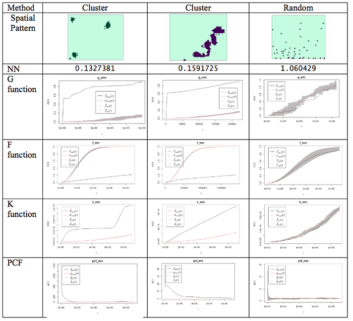
Figure 3.10 Examples of different spatial patterns and the results produced using the different distance-based analysis methods.
What do the plots show us?
Well, the dashed red line is the theoretical value of the function for a pattern generated by IRP/CSR. We aren't much interested in that, except as a point of reference.
The grey region (envelope) shows us the range of values of the function which occurred across all the simulated realizations of IRP/CSR which you see spatstat producing when you run the envelope function. The black line is the function for the actual pattern measured for the dataset.
What we are interested in is whether or not the observed (actual) function lies inside or outside the grey 'envelope'. In the case of the pair correlation function, if the black line falls outside the envelope, this tells us that there are more pairs of events at this range of spacings from one another than we would expect to occur by chance. This observation supports the view that the pattern is clustered or aggregated at the stated range of distances. For any distances where the black line falls within the envelope, this means that the PCF falls within the expected bounds at those distances. The exact interpretation of the relationship between the envelope and the observed function is dependent on the function in question, but this should give you the idea.
NOTE: One thing to watch out for... you may find that it's rather tedious waiting for 99 simulated patterns each time you run the envelope() function. This is the default number that are run. You can change this by specifying a different value for nsim. Once you are sure what examples you want to use, you will probably want to do a final run with nsim set to 99, so that you have more faith in the envelope generated (since it is based on more realizations and more likely to be stable). Also, you can change the rank setting. This will mean that the 'high' and 'low' lines in the plot will be placed at the corresponding high or low values in the range produced by the simulated realizations of IRP/CSR. So, for example:
> G_e <- envelope(xhomicide, Gest, nsim=99, nrank=5)will run 99 simulations and place high and low limits on the envelope at the 5th highest and 5th lowest values in the set of simulated patterns.
Something worth knowing is that the L function implemented in R deviates from that discussed in the text, in that it produces a result whose expected behavior for CSR is a upward-right sloping line at 45 degrees, that is expected L(r) = r, this can be confusing if you are not expecting it.
One final (minor) point: for the pair correlation function in particular, the values at short distances can be very high, and R will scale the plot to include all the values, making it very hard to see the interesting part of the plot. To control the range of values displayed in a plot, use xlim and ylim. For example:
> plot(pcf_env, ylim=c(0, 5))will ensure that only the range between 0 and 5 is plotted on the y-axis. Depending on the specific y-values, you may have to change the y-value in the ylim=() function.
Got all that? If you do have questions - as usual, you should post them to the Discussion Forum for this week's project. Also, go to the additional resources at the end of this lesson where I have included links to some articles that use some of these methods. Now, it is your turn to try this on the crime data you have been analyzing.
#Distance-based functions: G, F, K (and its relative L) and the more recent pair correlation function.  Gest(), Fest(), Kest(), Lest(), pcf()

#For this to run you may want to use a subset of the data otherwise you will find yourself waiting a long time.

g_env <-Gest(xhomicide)
plot(g_env)

#Add an envelope
#remember to change nsim=99 for the final simulation

#initializing and plotting the G estimation
g_env <-envelope(xhomicide, Gest, nsim=5, nrank=1)
plot(g_env)

#initializing and plotting the F estimation
f_env <- envelope(xhomicide, Fest, nsim=5, nrank=1)
plot(f_env)

#initializing and plotting the K estimation
k_env <-envelope(xhomicide, Kest, nsim=5, nrank=1)
plot(k_env)

#initializing and plotting the L estimation
l_env <- envelope(xhomicide, Lest, nsim=5, nrank=1)
plot(l_env)

#initializing and plotting the pcf estimation
pcf_env <-envelope(xhomicide, pcf, nsim=5, nrank=1)
# To control the range of values displayed in a plot's axes use xlim= and ylim= parameters
plot(pcf_env, ylim=c(0, 5))
Repeat this for the other crimes that you selected to analyze.
Project 3, Part B: Descriptive Spatial Statistics
Project 3, Part B: Descriptive Spatial StatisticsDescriptive Spatial Statistics
In Lesson 2, we highlighted some descriptive statistics that are useful for measuring geographic distributions. Additional details are provided in Table 3.3. Functions for these methods are also available in ArcGIS.
Table 3.3 Measures of geographic distributions that can be used to identify the center, shape and orientation of the pattern or how dispersed features are in space
| Spatial Descriptive Statistic | Description | Calculation |
|---|---|---|
| Central Distance | Identifies the most centrally located feature for a set of points, polygon(s) or line(s) | Point with the shortest total distance to all other points is the most central feature |
| Mean Center (there is also a median center called Manhattan Center) | Identifies the geographic center (or the center of concentration) for a set of features **Mean sensitive to outliers** | Simply the mean of the X coordinates and the mean of the Y coordinates for a set of points |
| Weighted Mean Center | Like the mean but allows weighting by an attribute. | Produced by weighting each X and Y coordinate by another variable (Wi) |
| Spatial Descriptive Statistic | Description | Calculation |
|---|---|---|
| Standard Distance | Measures the degree to which features are concentrated or dispersed around the geometric mean center The greater the standard distance, the more the distances vary from the average, thus features are more widely dispersed around the center Standard distance is a good single measure of the dispersion of the points around the mean center, but it doesn’t capture the shape of the distribution. | Represents the standard deviation of the distance of each point from the mean center: Where xi and yi are the coordinates for a feature and and are the mean center of all the coordinates. Weighted SD Where xi and yi are the coordinates for a feature and and are the mean center of all the coordinates. wi is the weight value. |
| Standard Deviational Ellipse | Captures the shape of the distribution. | Creates standard deviational ellipses to summarize the spatial characteristics of geographic features: Central tendency, Dispersion and Directional trends |
For this analysis, use the crime types that you selected earlier. The example here is for the homicide data.
#------MEAN CENTER
#calculate mean center of the crime locations
xmean <- mean(xhomicide$x)
ymean <-mean(xhomicide$y)

#------MEDIAN CENTER
#calculate the median center of the crime locations
xmed <- median(xhomicide$x)
ymed <- median(xhomicide$y)

#to access the variables in the shapefile, the data needs to be set to data.frame
newhom_df<-data.frame(xhomicide)
#check the definition of the variables.
str(newhom_df)

#If the variables you are using are defined as a factor then convert them to an integer
newhom_df$FREQUENCY <- as.integer(newhom_df$FREQUENCY)
newhom_df$OBJECTID <- as.integer(newhom_df$OBJECTID)

#create a list of the x coordinates. This will be used to define the number of rows
a=list(xhomicide$x)


#------WEIGHTED MEAN CENTER
#Calculate the weighted mean
d=0
sumcount = 0
sumxbar = 0
sumybar = 0
for(i in 1:length(a[[1]])){
  xbar <- (xhomicide$x[i] * newhom_df$FREQUENCY[i])
  ybar <- (xhomicide$y[i] * newhom_df$FREQUENCY[i])
  sumxbar = xbar + sumxbar
  sumybar = ybar + sumybar
  sumcount <- newhom_df$FREQUENCY[i]+ sumcount
}
xbarw <- sumxbar/sumcount
ybarw <- sumybar/sumcount


#------STANDARD DISTANCE OF CRIMES
# Compute the standard distance of the crimes
#Std_Dist <- sqrt(sum((xhomicide$x - xmean)^2 + (xhomicide$y - ymean)^2) / nrow(xhomicide$n))

#Calculate the Std_Dist
d=0
for(i in 1:length(a[[1]])){
  c<-((xhomicide$x[i] - xmean)^2 + (xhomicide$y[i] - ymean)^2)
  d <-(d+c)
}
Std_Dist <- sqrt(d /length(a[[1]]))

# make a circle of one standard distance about the mean center
bearing <- 1:360 * pi/180
cx <- xmean + Std_Dist * cos(bearing)
cy <- ymean + Std_Dist * sin(bearing)
circle <- cbind(cx, cy)


#------CENTRAL POINT
#Identify the most central point:
#Calculate the point with the shortest distance to all points
#sqrt((x2-x1)^2 + (y2-y1)^2

sumdist2 = 1000000000
for(i in 1:length(a[[1]])){
  x1 = xhomicide$x[i]
  y1= xhomicide$y[i]
  recno = newhom_df$OBJECTID[i]
  #print(recno)
  #check against all other points
    sumdist1 = 0
    for(j in 1:length(a[[1]])){
      recno2 = newhom_df$OBJECTID[j]
      x2 = xhomicide$x[j]
      y2= xhomicide$y[j]
      if(recno==recno2){
      }else {
      dist1 <-(sqrt((x2-x1)^2 + (y2-y1)^2))
         sumdist1 = sumdist1 + dist1
         #print(sumdist1)
         }
    }
    #print("test")
    if (sumdist1 < sumdist2){
           dist3<-list(recno, sumdist1, x1,y1)
           sumdist2 = sumdist1
           xdistmin <- x1
           ydistmin <- y1
         }
}

#------MAP THE RESULTS
#Plot the different centers with the crime data
plot(Sbnd)
points(xhomicide$x, xhomicide$y)
points(xmean,ymean,col="red", cex = 1.5, pch = 19) #draw the mean center
points(xmed,ymed,col="green", cex = 1.5, pch = 19) #draw the median center
points(xbarw,ybarw,col="blue", cex = 1.5, pch = 19) #draw the weighted mean center
points(dist3[[3]][1],dist3[[4]][1],col="orange", cex = 1.5, pch = 19) #draw the central point
lines(circle, col='red', lwd=2)
Deliverable
Perform point pattern analysis on any two of the available crime datasets (DUI, arson, or homicide). It would be beneficial if you would choose crimes with contrasting patterns. For your analysis, you should choose whatever methods seem the most useful, and present your findings in the form of maps, graphs, and accompanying commentary.
Project 3: Finishing Up
Project 3: Finishing UpPlease upload your write-up Project 3 Drop Box.
Deliverables
For Project 3, the items you are required to submit are as follows:
- First, create figures of the different point patterns you generated in Part A according to different random processes with accompanying commentary that explains the patterns that were created
- Second, create density maps of three of the available crime datasets (homicide + 2 of your choice) , experimenting with the kernel density bandwidth, and provide a commentary discussing the most suitable bandwidth choice for this analysis visualization method.
- Third, perform point pattern analyses in Part B on three of the available crime datasets (homicide + 2 of your choice). It would be beneficial if you would choose crimes with contrasting patterns. Crimes with low counts will not produce very compelling patterns and the analysis techniques will not be meaningful.
- Use the questions below to help you think about and synthesize the results from the various analyses you completed in this project:
- What were your overall findings about crime in your study area?
- Where did crimes take place? Was there a particular spatial distribution associated with each of the crimes? Did they take place in a particular part of the city?
- Did the different crimes you assessed cluster in different parts of the study area or did they occur in the same parts of the city?
- What additional types of analysis would be useful?
- Another part of spatial analysis is centered on ethical considerations about the data, which include but are not limited to: who collected the data and what hidden (or overt) messages are contained within the data?
- Consider that the St. Louis dataset contains roughly a year's worth of crime data leading up to the protests that took place in Ferguson, MO during August 2014. Here is one news reporting of that event.
- Data are inherently contrived by the individuals and organizations that collect, format, and then make data available for use.
- As the analyst for this project, comment on the ethical considerations that you should take when formatting, analyzing, and reporting the results for Lesson 3? Knowing that the data included possible events leading up to the Ferguson protests, what kinds of decisions would you make in analyzing the data in Lesson 2?
- Remember that data is not simply binary or a listing of numbers, but can be a complex set of biases and injustices that may be opaque to the user.
That's it for Project 3!
Afterword
AfterwordNow that you are finished with this week's project, you may be interested to know that some of the tools you've been using are available in ArcGIS. You will find mean nearest neighbor distance and Ripley's K tools in the Spatial Statistics - Analyzing Patterns toolbox. The Ripley's K tool in particular has improved significantly since ArcGIS 10, so that it now includes the ability to generate confidence envelopes using simulation, just like the envelope() function in R.
For kernel density surfaces, there is a density estimation tool in the Spatial Analyst Tools - Density toolbox. This is essentially the same as the density() tool in R with one very significant difference, namely that Arc does not correct for edge effects.
In Figure 3.11 the results of kernel density analysis applied to all the crime events in the project data set are shown for (from left to right) the default settings in ArcGIS, with a mask and processing extent set in ArcGIS to cover the city limits area, and for R.

Figure 3.11: Three KDE using the default settings on the three crime data sets.
The search radius in ArcGIS was set to 2 km and the 'sigma' parameter in R was set to 1 km. These parameters should give roughly equivalent results. More significant than the exact shape of the results is that R is correcting for edge effects. This is most clear at the north end of the map, where R's output implies that the region of higher density runs off the edge of the study area, while ArcGIS confines it to the analysis area. R accomplishes this by basing its density estimate on only the bandwidth area inside the study area at each location.
Descriptive Spatial Statistics in ArcGIS:
The descriptive spatial statistics tools can be found in the Spatial Statistics – Measuring Geographic Distributions toolbox in ArcToolbox. To do this analysis for different crime types or different time periods (year, month) set the case field.
The extensibility of both packages makes it to some extent a matter of taste which you choose to use for point pattern analysis. It is clear that R remains the better choice in terms of the range of available options and tools, although ArcGIS may have the edge in terms of its familiarity to GIS analysts. For users starting with limited knowledge of both tools, it is debatable which has the steeper learning curve - certainly neither is simple to use!
Term Project (Week 3): Peer review group meeting info
Term Project (Week 3): Peer review group meeting infoThe project this week is quite demanding, so there is no set deliverable this week.
Continue to refine your project proposal. In a separate announcement, information about the peer review group membership will be sent. Once you know your group memeber, you can communicate with them and set a day and time to meet.
Additional details can be found on the Term Project Overview Page.
Questions?
Please use the 'Discussion - General Questions and Technical Help' discussion forum in Canvas to ask any questions now or at any point during this project.
Final Tasks
Final TasksLesson 3 Deliverables
- Complete the Lesson 3 quiz.
- Complete the Project 3A and 3B activities. This includes inserting maps and graphs into your write-up along with accompanying commentary. Submit your assignment to the 'Assignment: Week 3 Project' dropbox provided in Lesson 3 in Canvas.
Reminder - Complete all of the Lesson 3 tasks!
You have reached the end of Lesson 3! Double-check the to-do list on the Lesson 3 Overview page to make sure you have completed all of the activities listed there before you begin Lesson 4.
References and Additional Resources
For additional information about spatstat refer to this document by Baddeley
To see how some of these methods are applied, have a quick look at some of these journal articles.
Here is an article to an MGIS capstone project that investigated sinkholes in Florida.
Related to crime, here is a link to an article that uses spatial analysis for understanding crime in national forests.
Here's an article that uses some of the methods learned during this week's lesson to analyze the distribution of butterflies within a heterogeneous landscape.
For a comprehensive read on using crime analysis, look through Crime Modeling and Mapping Using Geospatial Technologies book available through the Penn State Library.
Don't forget to use the library and search for other books or articles that may be applicable to your studies.