The central class of the API is the GIS class defined in the arcgis.gis module. It represents the GIS you are working with to access and publish content or to perform different kinds of management or analysis tasks. A GIS object can be connected to AGOL or Enterprise/Portal for ArcGIS. Typically, the first step of working with the API in a Python script consists of constructing a GIS object by invoking the GIS(...) function defined in the argis.gis module. There are many different ways of how this function can be called, depending on the target GIS and the authentication mechanism that should be employed. Below we are showing a couple of common ways to create a GIS object before settling on the approach that we will use in this class, which is tailored to work with your pennstate organizational account.

Most commonly, the GIS(...) function is called with three parameters, the URL of the ESRI web GIS to use (e.g. ‘https://www.arcgis.com’ for a GIS object that is connected to AGOL), a username, and the login password of that user. If no URL is provided, the default is ArcGIS Online, and it is possible to create a GIS object anonymously without providing username and password. So the simplest case would be to use the following code to create an anonymous GIS object connected to AGOL (we do not recommend running this code - it is shown only as an example):

from arcgis.gis import GIS
gis = GIS()

Due to not being connected to a particular user account, the available functionality will be limited. For instance, you won’t be able to upload and publish new content. If, instead, you'd want to create the GIS object but with a username and password for a normal AGOL account (so not an enterprise account), you would use the following way with <your username> and <your password> replaced by the actual username and password (we do not recommend running this code either. It is shown only as an example):

from arcgis.gis import GIS
gis = GIS('https://www.arcgis.com', '<your username>', '<your password>')
gis?

This approach unfortunately does not work with the pennstate organizational account you had to create at the beginning of the class. But we will need to use this account in this lesson to make sure you have the required permissions. You already saw how to connect with your pennstate organizational account if you tried out the test code in Section 3.2. The URL needs to be changed to ‘https://pennstate.maps.arcgis.com’ and we have to use a parameter called client_id to provide the ID of an app that we created for this class on AGOL. When using this approach, calling the GIS(...) function will open a browser window where you can authenticate with your PSU credentials and/or you will be asked to grant the permission to use Python with your pennstate AGOL account. After that, you will be given a code that you have to paste into a box that will be showing up in your notebook. The details of what is going on behind the scenes are a bit complicated but whenever you need to create a GIS object in this class to work with the API, you can simply use these exact few lines and then follow the steps we just described. The last line of the code below is for testing that the GIS object has been created correctly. It will print out some help text about the GIS object in a window at the bottom of the notebook. The screenshot below illustrates the steps needed to create the GIS object and the output of the gis? command. (for safety it would be best to restart your Notebook kernel prior to running the code below if you did run the code above as it can cause issues with the below instructions working properly)

The token issued by this process is short-lived and does not give the user any indication that it has expired. If you start seeing errors such as "TypeError: 'Response' object is not subscriptable" or "Exception: A general error occurred: 'Response' object is not subscriptable" when running your Notebook and the stack trace contains "Connection.post", "EsriSession.post", "EsriOAuth2Auth.__call__(self, r)", "EsriOAuth2Auth._oauth_token(self)" in the stack trace, execute the GIS(...) sign in process and try the cell again.

import arcgis
from arcgis.gis import GIS
gis = GIS('https://pennstate.maps.arcgis.com', client_id='fuFmRsy8iyntv3s2')
gis?

Figure 3.18 Steps for creating GIS object and output produced by the gis? command in the previous code example

Note about the paste window: This varies between IDE. For VS Code, it is very subtle popup that appears at the top of the IDE after you run the cell. PyCharm provides an input line in a popup, and other IDE's may use other windows to prompt for the input.

The GIS object in variable gis gives you access to a user manager (gis.users), a group manager (gis.groups) and a content manager (gis.content) object. The first two are useful for performing administrative tasks related to groups and user management. If you are interested in these topics, please check out the examples on the Accessing and Managing Users and Batch Creation of Groups pages. Here we simply use the get(...) method of the user manager to access information about a user, namely ourselves. Again, you will have to replace the <your username> tag with your PSU AGOL name to get some information display related to your account:

user = gis.users.get('<your username>')
user

The user object now stored in variable user contains much more information about the given user in addition to what is displayed as the output of the previous command. To see a list of available attributes, type in

user.

and then press the TAB key for the Jupyter autocompletion functionality. The following command prints out the email address associated with your account:

user.email

We will talk about the content manager object in a moment. But before that, let’s talk about maps and how easy it is to create a web map like visualization in a Jupyter Notebook with the ArcGIS API. A map can be created by calling the map(...) method of the GIS object. We can pass a string parameter to the method with the name of a place that should be shown on the map. The API will automatically try to geocode that name and then set up the parameters of the map to show the area around that place. Let’s use State College as an example:

map = gis.map('State College, PA')
map

Figure 3.19 Map widget in Jupyter Notebook produced by the previous code example

The API contains a widget for maps so that these will appear as an interactive map in a Jupyter Notebook. As a result, you will be able to pan around and use the buttons at the top left to zoom the map. The map object has many properties and methods that can be used to access its parameters, affect the map display, provide additional interactivity, etc. For instance, the following command changes the zoom property to include a bit more area around State College. The map widget will automatically update accordingly.

map.zoom = 11

With the following command, we change the basemap tiles of our map to satellite imagery. Again the map widget automatically updates to reflect this change.

map.basemap.basemap = 'satellite'

As another example, let’s add two simple circle marker objects to the map, one for Walker Building on the PSU campus, the home of the Geography Department, and one for the Old Main building. The ArcGIS API provides a very handy geocode(...) function in the arcgis.geocoding module so that we won’t have to type in the coordinates of these buildings ourselves. The properties of the marker are defined in the pt_sym dictionary.

#add features
from arcgis.geocoding import geocode
from arcgis.features import Feature, FeatureSet
# Define the point symbol
pt_sym = {
    "type": "esriSMS",
    "style": "esriSMSCircle",
    "color": [255, 0, 0, 255],  # Red color
    "size": 10
}

# Geocode addresses
walker = geocode('Walker Bldg, State College, PA')[0]
oldMain = geocode('Old Main Bldg, State College, PA')[0]

# Add spatial reference to the geometries (WGS84, WKID: 4326)
walker['location']['spatialReference'] = {"wkid": 4326}
oldMain['location']['spatialReference'] = {"wkid": 4326}

# Create point features with attributes
walker_feature = Feature(geometry=walker['location'], attributes={"Name": "Walker Bldg", "Label": walker['attributes']['LongLabel']})
oldMain_feature = Feature(geometry=oldMain['location'], attributes={"Name": "Old Main Bldg", "Label": oldMain['attributes']['LongLabel']})

# Create a FeatureSet with both points
features = FeatureSet([walker_feature, oldMain_feature])

# Draw the features on the map with the specified symbol
map.content.add(features, {"renderer": {"type": "simple", "symbol": pt_sym}})

Figure 3.20 Map widget in Jupyter Notebook produced by the previous code example

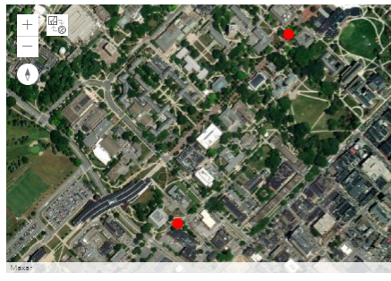
The map widget should now include the markers for the two buildings as shown in the image above (the markers may look different). A little explanation on what happens in the code: the geocode(...) function returns a list of candidate entities matching the given place name or address, with the candidate considered most likely appearing as the first one in the list. We here simply trust that the ArcGIS API has been able to determine the correct candidate and hence just take the first object from the respective lists via the “[0]” in the code. What we now have stored in variables walker and oldMain are dictionaries with many attributes to describe the entities. We create Features and then a FeatureSet to be added to the map.

Now let’s get back to the content manager object of our GIS. The content manager object allows us to search and use all the content we have access to. That includes content we have uploaded and published ourselves but also content published within our organization and content that is completely public on AGOL. Content can be searched with the search(...) method of the content manager object. The method takes a query string as parameter and has additional parameters for setting the item type we are looking for and the maximum number of entries returned as a result for the query. For instance, try out the following command to get a list of available feature services that have PA in the title:

featureServicesPA = gis.content.search(query='title:PA', item_type='Feature Layer Collection', max_items = 25)
featureServicesPA

This will display a list of different AGOL feature service items available to you. The list is probably rather short at the moment because not much has been published in the new pennstate organization yet, but there should at least be one entry with municipality polygons for PA. Each feature service from the returned list can, for instance, be added to your map or used for some spatial analysis. To add a feature service to your map as a new layer, you have to use the add(...) method of the map.content like we did above. For example, the following command takes the first feature service from our result list in variable featureServicesPA and adds it to our map widget:

map.content.add(featureServicesPA[0], {'opacity': 0.8})

The first parameter specifies what should be added as a layer (the feature service with index 0 from our list in this case), while the second parameter is an optional dictionary with additional attributes (e.g., opacity, title, visibility, symbol, renderer) specifying how the layer should be symbolized and rendered. Feel free to try out a few other queries (e.g. using "*" for the query parameter to get a list of all available feature services) and adding a few other layers to the map by changing the index used in the previous command. If the map should get too cluttered, you can simply recreate the map widget with the map = gis.map(...) command from above.

The query string given to search(...) can contain other search criteria in addition to ‘title’. For instance, the following command lists all feature services that you are the owner of (replace <your agol username> with your actual Penn State AGOL/Pro username):

gis.content.search(query='owner:<your agol username>', item_type='Feature Service')

Unless you have published feature services in your AGOL account, the list returned by this search will most likely be empty ([]). So how can we add new content to our GIS and publish it as a feature service? That’s what the add(...) method of the content manager object and the publish(...) method of content items are for. The following code uploads and publishes a shapefile of larger cities in the northeast of the United States.

To run it, you will need to first download the zipped shapefile and then slightly change the filename on your computer. Since AGOL organizations must have unique services names, edit the file name to something like ne_cities_[initials].zip or ne_cities_[your psu id].zip so the service name will be unique to the organization. Adapt the path used in the code below to refer to this .zip file on your disk.

# get the root folder of the user
root_folder = gis.content.folders.get()

# Ensure the folder is found
if root_folder:
    # Add the shapefile to the folder
    shapefile_path = r"C:\489\L3\ne_cities_test.zip"
    # Add the zip to the AGOL
    neCities = root_folder.add({"title": "ne_cities_test", "type": "Shapefile"}, shapefile_path).result()

    # Print the result
    print(f"Shapefile added to folder: {neCities.title}")
    neCitiesFS = neCities.publish()
    display(neCitiesFS)
    print(f"{neCities.title} published as a service")
else:
    print("Folder not found")

The api needs to upload the shapefile to a folder, and the code above uses the root folder of the user. If you had a specific folder you wanted to upload the shapefile to, you can get or set the folder name. It is important to note that the shapefile upload is done asynchronously, and the .result() at the end of the add method call tells the execution to wait for the upload to finish before moving on. Without this, or without waiting for the result object to return, neCities will be None and cause further execution errors.

The first parameter given to gis.content.add(...) is a dictionary that can be used to define properties of the data set that is being added, for instance tags, what type the data set is, etc. Variable neCitiesFS now refers to a published content item of type arcgis.gis.Item that we can add to a map with add(...). There is a very slight chance that this layer will not load in the map. If this happens for you - continue and you should be able to do the buffer & intersection operations later in the walkthrough without issue. Let’s do this for a new map widget:

cityMap = gis.map('Pennsylvania')
cityMap.content.add(neCitiesFS, {})
cityMap

Figure 3.21 Map widget produced by the previous code example

The image shows the new map widget that will now be visible in the notebook. If we rerun the query from above again...

gis.content.search(query='owner:<your agol username>', item_type='Feature Service')

...our newly published feature service should now show up in the result list as:

<Item title:"ne_cities" type:Feature Layer Collection owner:<your AGOL username>>

The ArcGIS Python API also provides the functionality to access individual features in a feature layer, to manipulate layers, and to run analyses from a large collection of GIS tools including typical GIS geoprocessing tools. Most of this functionality is available in the different submodules of arcgis.features. To give you a few examples, let’s continue with the city feature service we still have in variable neCitiesFS from the previous section. A feature service can actually have several layers but, in this case, it only contains one layer with the point features for the cities. The following code example accesses this layer (neCitiesFE.layers[0]) and prints out the names of the attribute fields of the layer by looping through the ...properties.fields list of the layer:

for f in neCitiesFS.layers[0].properties.fields:
	print(f)

When you try this out, you should get a list of dictionaries, each describing a field of the layer in detail including name, type, and other information. For instance, this is the description of the STATEABB field:

{
 "name": "STATEABB",
 "type": "esriFieldTypeString",
 "actualType": "nvarchar",
 "alias": "STATEABB",
 "sqlType": "sqlTypeNVarchar",
 "length": 10,
 "nullable": true,
 "editable": true,
 "domain": null,
 "defaultValue": null
 }

The query(...) method allows us to create a subset of the features in a layer using an SQL query string similar to what we use for selection by attribute in ArcGIS itself or with arcpy. The result is a feature set in ESRI terms. If you look at the output of the following command, you will see that this class stores a JSON representation of the features in the result set. Let’s use query(...) to create a feature set of all the cities that are located in Pennsylvania using the query string "STATEABB"='US-PA' for the where parameter of query(...):

paCities = neCitiesFS.layers[0].query(where='"STATEABB"=\'US-PA\'')
print(paCities.features)
paCities

Output: 
[{"geometry": {"x": -8425181.625237303, "y": 5075313.651659228}, 
"attributes": {"FID": 50, "OBJECTID": "149", "UIDENT": 87507, "POPCLASS": 2, "NAME": 
"Scranton", "CAPITAL": -1, "STATEABB": "US-PA", "COUNTRY": "USA"}}, {"geometry": 
{"x": -8912583.489066456, "y": 5176670.443556941}, "attributes": {"FID": 53, 
"OBJECTID": "156", "UIDENT": 88707, "POPCLASS": 3, "NAME": "Erie", "CAPITAL": -1, 
"STATEABB": "US-PA", "COUNTRY": "USA"}}, ...  ]
<FeatureSet> 10 features

Of course, the queries we can use with the query(...) function can be much more complex and logically connect different conditions. The attributes of the features in our result set are stored in a dictionary called attributes for each of the features. The following loop goes through the features in our result set and prints out their name (f.attributes['NAME']) and state (f.attributes['STATEABB']) to verify that we only have cities for Pennsylvania now:

for f in paCities:
	print(f.attributes['NAME'] + " - "+ f.attributes['STATEABB'])

Output: 
Scranton - US-PA
Erie - US-PA
Wilkes-Barre - US-PA
...
Pittsburgh - US-PA

Now, to briefly illustrate some of the geoprocessing functions in the ArcGIS Python API, let’s look at the example of how one would determine the parts of the Appalachian Trail that are within 30 miles of a larger Pennsylvanian city. For this we first need to upload and publish another data set, namely one that’s representing the Appalachian Trail. We use a data set that we acquired from PASDA for this, and you can download the DCNR_apptrail file here. As with the cities layer earlier, there is a very small chance that this will not display for you - but you should be able to continue to perform the buffer and intersection operations. The following code uploads the file to AGOL (don’t forget to adapt the path and add your initials or ID to the name!), publishes it, and adds the resulting trail feature service to your cityMap from above:

# change this variable to the name of the zip file and service
dcnr_file = "dcnr_apptrail_2003_???"
appTrail = rf'C:\PSU\Geog 489\Lesson 3\Notebooks\{dcnr_file}.zip'

# test if it exists in AGOL first
appTrailshp_test = gis.content.search(query=f'owner:{user_name} title:{dcnr_file}', item_type='Feature Layer Collection')

if appTrailshp_test:
    appTrailFS = appTrailshp_test[0]
    print(f"{appTrailFS.title} found in AGOL")
else:
    root_folder = gis.content.folders.get()
    # Ensure the folder is found
    if root_folder:       
        # Add the shapefile to the folder.
        appTrailshp = root_folder.add({"title": dcnr_file, "type": "Shapefile"}, appTrail).result()
    
        # Print the result
        print(f"Shapefile added to folder: {appTrailshp.title}")
        appTrailFS = appTrailshp.publish()
        print(f"{appTrailFS.title} published as a service")
    else:
        print("Folder not found")

display(appTrailFS)

cityMap.content.add(appTrailFS, {})

cityMap

Figure 3.23 Map widget now showing the cities and trail layers

Let's take a moment to talk about credits. Credits are what esri uses to charge users for certain processing tasks and storage in AGOL. Processes such as geocoding, clipping, routing, buffering, or storing data and content costs the organization credits. More details can be found in esri's documentation here, and it is important to protect your account credentials so someone does not drain your credits (among other things). The rest of the walkthrough performs tasks that costs credits, so we include preliminary code that checks if the result exist in AGOL before executing the geoprocessing step. When you first run the blocks below, it will create the data in AGOL since it most likely does not exist. Subsequent executions (who executes a script just once?) it will find and use the existing data from a previous run, saving your credits.

Next, we create a 30 miles buffer around the cities in variable paCities that we can then intersect with the Appalachian Trail layer. The create_buffers(...) function that we will use for this is defined in the arcgis.features.use_proximity module together with other proximity based analysis functions. We provide the feature set we want to buffer as the first parameter, but, since the function cannot be applied to a feature set directly, we have to invoke the to_dict() method of the feature set first. The second parameter is a list of buffer distances allowing for creating multiple buffers at different distances. We only use one distance value, namely 30, here and also specify that the unit is supposed to be ‘Miles’. Finally, we add the resulting buffer feature set to the cityMap above.

This operation costs credits so once it is created in AGOL, try not to delete it unless absolutely necessary.

The title is used for the output_name so it can be found in AGOL after initial creation.

# 
from arcgis.features.use_proximity import create_buffers
import urllib3

title = 'bufferedCities_???'

# test if it exists in AGOL first
bufferedCities_test = gis.content.search(query=f'owner:{user_name} title:{title}', item_type='Feature Layer Collection')

if bufferedCities_test:
    bufferedCities = bufferedCities_test[0]
    print(f"{bufferedCities.title} found in AGOL")
else:
    # Disable SSL warnings (or it will print a lot of them)
    urllib3.disable_warnings(urllib3.exceptions.InsecureRequestWarning)
    
    bufferedCities = create_buffers(paCities.to_dict(), [30], units='Miles', output_name=title)
    
    # Print the result
    print(f"Shapefile added to folder: {bufferedCities.title}")

cityMap.content.add(bufferedCities, {})

Figure 3.24 Map widget with buffers created by the previous code example

As the last step, we use the overlay_layers(...) function defined in the arcgis.features.manage_data module to create a new feature set by intersecting the buffers with the Appalachian Trail polylines. For this we have to provide the two input sets as parameters and specify that the overlay operation should be ‘Intersect’.

This operation costs credits so once it is created in AGOL, try not delete it unless absolutely necessary.

The title is used for the output_name so it can be found in AGOL after initial creation.

# 
from arcgis.features.analysis import overlay_layers
# OR from arcgis.features.manage_data import overlay_layers which does the same
title = 'city_trailhead_???'

# test if it exists in AGOL first
trailPartsCloseToCity_test = gis.content.search(query=f'owner:{user_name} title:{title}', item_type='Feature Layer Collection')

if trailPartsCloseToCity_test:
    trailPartsCloseToCity = trailPartsCloseToCity_test[0]
    print(f"{trailPartsCloseToCity.title} found in AGOL")
else:
    # Perform the overlay (Intersection)
    trailPartsCloseToCity = overlay_layers(appTrailFS.layers[0], bufferedCities.layers[0], overlay_type='Intersect', output_name=title)
    print(f"{trailPartsCloseToCity.title} created")
    
# Check the result
print(trailPartsCloseToCity)

We show the result by creating a new map ...

# 
resultMap = gis.map('Pennsylvania')

... and just add the features from the resulting trailPartsCloseToCity feature set to this map:

# 
resultMap.content.add(trailPartsCloseToCity, {})

resultMap

The result is shown in the figure below.

Figure 3.25 New map widget showing the final result of our analysis

This section gave you a brief introduction to ESRI's ArcGIS API for Python and showed you some of the most important methods and patterns that you will typically encounter when using the API. The API is much too rich to cover everything here, so, to get a better idea of the geoprocessing and other capabilities of the API, we recommend that you check and try out some of the sample notebooks that ESRI has published, such as:

• Chennai Floods 2015 - a geographic analysis
• Fighting California forest fires using spatial analysis

A lot of valuable information can also be gained from the ESRI's API guide, and, of course, the API documentation.