Unit 3: Social Science of Water
Unit 3: Social Science of WaterOverview
Congratulations! You have completed the first two units of the "Water: Science and Society" course. Having done so, you are prepared to tackle some serious issues with respect to fresh-water resources, both in the U.S. and globally. Unit 3 comprises four modules (7-10) that are spread over five weeks of the semester. These modules present an overview of the water supply challenges that face society now and in the future, and prompt you to explore possible solutions to those challenges.
Module 7 ("What's In Your Water?") delves into the role of water as a "universal solvent" and the problems that its ability to dissolve and transport nearly any potential chemical pollutant present for drinking water quality, water quality in natural environments, and agricultural activities. The module offers several short "case studies" whereby human activities alter the chemistry of surface- and/or groundwater, creating toxic conditions for humans and wildlife (e.g., so-called "dead zones" in coastal regions), and asks you to consider possible solutions to these and other water quality problems through regulation or process changes.
Module 8 ("Cities in Peril: Dealing with Water Scarcity, Part 1: History and Current Approaches, and Part 2: Future Growth and Climate Change") covers two weeks of the course and focuses on the problems of major population centers with respect to acquiring clean drinking water. Understandably, the problem is more extreme for large cities located in arid regions (e.g., Los Angeles, CA or Las Vegas, NV), but is not governed simply by water availability. Infrastructure construction and maintenance is another related issue. There is also strong pressure on fresh water availability from prolonged drought, which could result from global climate change. The second part of Module 8 introduces climate change as a factor, what we understand now, and how well we can predict future changes.
In Module 9 ("Water and Politics: International Issues") we entertain the human penchant for laying claim to water resources, and the need to fairly "share" resources in cases where rivers (or groundwater basins) cross international borders (or in some cases, rivers that are the basis for international borders), while also protecting water quality. Are old treaties adequate as governments change and populations grow? Will we experience further "water wars?" The Nile River in northeast Africa and the Colorado River in western North America are good examples.
Module 10 ("Solving the Water Crisis? Potential Solutions to Problems with Water Scarcity and Quality") is the culmination of the course, bringing together diplomacy, economics, and technology to explore potential solutions for fresh water shortages. Some of these solutions, although elegant and high-tech, will not be feasible where funding and energy are in short supply. You will evaluate these possibilities and recommend a path forward.
Modules
- Module 7: What Is In Your Water?
- Module 8: Cities in Peril: Dealing with Water Scarcity
- Module 9: Water and Politics: Global Issues
- Module 10: Solving the Water Crisis?
Unit Goals
Upon completion of Unit 3 students will be able to:
- Describe the two-way relationship between water resources and human society.
- Explain the distribution and dynamics of water at the surface and in the subsurface of the Earth.
- Synthesize data and information from multiple reliable sources.
- Interpret graphical representations of scientific data.
- Identify strategies and best practices to decrease water stress and increase water quality
- Thoughtfully evaluate information and policy statements regarding water resources
- Communicate scientific information in terms that can be understood by the general public
- Predict how the availabilty of and demand for water resources is expected to change over the next 50 years
Module 7: What is in Your Water?
Module 7: What is in Your Water?Overview
Water is the "Universal Solvent." Virtually every element on the periodic table and many organic substances (molecules) are soluble (can be dissolved) to some degree in water. Many substances occur "naturally" in water—that is they are dissolved into water as it flows over rock surfaces or through aquifers in the subsurface or as it mixes with other waters. Some substances are "pollutants," having been added as the result of certain human activities, intentionally or unintentionally, including wastewater (untreated) disposal, drainage of acidic waters from abandoned mines, drainage from agricultural operations (e.g. manure, herbicides, pesticides), etc. "Water quality" implies an assessment of the degree of contamination of a water source by direct measurement of its dissolved components. Not all dissolved components in water are harmful to human health, but this depends, in part, on their concentration. In this module, we will explore some of the science and issues with respect to drinking water quality, a bit about the chemistry of natural waters, and the regulations that help ensure a satisfactory drinking water supply for the U.S. populace. In addition, we will outline some water quality issues that affect other parts of the globe.
Goals and Objectives
Goals and ObjectivesGoals
- Describe the two-way relationship between water resources and human society
- Explain the distribution and dynamics of water at the surface and in the subsurface of the Earth
- Synthesize data and information from multiple reliable sources
- Interpret graphical representations of scientific data
- Identify strategies and best practices to decrease water stress and increase water quality
- Thoughtfully evaluate information and policy statements regarding water resources
- Communicate scientific information in terms that can be understood by the general public
Learning Objectives
In completing this module, you will:
- Calculate the concentration of contaminant in a reservoir
- Apply government drinking water regulatory standards to identify contaminant levels that might be harmful to human health
- Analyze concentration vs. time data for various dissolved components of river water and ground water
- Infer the processes responsible for seasonal trends in compounds of natural and human origin
- Propose and evaluate methods for mitigating human impacts on water quality
- Evaluate the tradeoff between agricultural productivity and water quality as a result of fertilizer usage and runoff
Units of Water Chemistry
Units of Water ChemistryElements and molecules have solubilities (the amount that can be dissolved in water before the water is saturated with that element and no more can be held in solution) that depend on their individual properties and styles of bonding to other elements. For example, common table salt (NaCl), when added to water, will dissociate into individual charged ions of Na+ and Cl-. These are held apart from one another "in solution" because they are surrounded and isolated by polar water molecules (Unique Properties of Water section).
Distilled water or "pure" water typically has near-zero concentrations of other components. If concentrations of dissolved elements or compounds are present, they are usually expressed in terms of mass (weight) of the component/unit volume of water, mass element/mass water, or moles element/mass or volume of water.
Typically, the volume of water referenced is a liter (1000 grams--1 kg by mass), and the elemental or component mass is in grams (or milligrams, mg). Milligrams/Liter (mg/L; 0.001g/1000g) or milligrams/kg (mg/kg) is the same as parts per million (ppm) as concentration. You will often see a concentration of a dissolved species in water expressed in either mg/L or ppm.
Molar concentrations, commonly used by chemists, are expressed as a decimal fraction of the mass of Avogadro's Number (a mole) of atoms (6.022 x 10²³) of a given element or elements in a compound, equivalent to atomic or molecular mass. For example, a mole of carbon (12C) has a mass of 12 grams, and a mole of carbon dioxide (CO2) has a mass of 44 grams (12C, 16O, 16O). So, if a liter water sample contains 0.044g of carbon dioxide (44 ppm), the carbon dioxide concentration would be 0.01 mole/kg.
Learning Checkpoint
1. The Na concentration in a water sample is 10 ppm. What is the concentration expressed in g/kg?
2. The mass of a mole of sodium (Na) is about 23 g. A water sample has a dissolved sodium concentration of 0.046 g/kg. What is the Na concentration expressed as moles/L?
3. Read this article about a contaminated water supply. After mixing in with the 38 million gallons of fresh water already in the reservoir, how many parts per million “contaminant” are there (in other words, what is the proportion of the contaminated water to the total volume)? Assume that the input of “contaminant” is 8 oz.
Drinking Water Regulation
Drinking Water RegulationWho Regulates Drinking Water Quality in the U.S.?
Public drinking water quality is regulated by the U.S. Environmental Protection Agency (EPA) by provisions of the Safe Drinking Water Act (SDWA), although individual states can apply and enforce their own standards if more stringent than those set by the EPA. The SDWA was originally passed by the U.S. Congress in 1974, and has been amended twice (1986, 1996) and now provides standards for drinking-water sources, treatment, and quality at the tap, as well as the disposal of wastewater underground. Private wells pumping groundwater that serve fewer than 25 people are not regulated. They should be tested regularly, however.
It is estimated that there are over 160,000 public drinking-water systems that fall under the aegis of the EPA standards. These standards are health-based and attempt to establish maximum levels (MCL—Maximum Contaminant Level) for possible contaminants that are below those that are thought to cause health problems (you can see specific contaminants and MCLs at EPA: Drinking Water Contaminants - Standards and Regulations). Of course, there are many contaminants for which there are insufficient data to establish stringent limits.
Over the past decade, bottled water, usually sealed in "plastic" containers has become quite popular worldwide. Accoring to bottledwater.org, in the U.S., over 15.9 billion gallons of bottled water were sold in 2022, revenues were more than $46 billion, assuming an average price of $1 per liter. Although convenience is certainly a factor, the perception has been that such water must be safe to drink—perhaps more safe than tap water—also drives bottled water sales. In the U.S., bottled water is actually regulated by the U.S. Food and Drug Administration (FDA), not the EPA. The FDA regulates bottled water as a food (requiring compliance with the Federal Food, Drug and Cosmetic Act) and does not require certified lab testing or violation reporting, even though the FDA does inspect bottling plants and ensures that suitable source waters are used. The FDA also has generally adopted limits for contaminants established by the EPA. Nonetheless, the FDA does not require bottled water companies to disclose to consumers the source of the water, treatment processes, or contaminants it contains, whereas the EPA requires public water systems to report results of their testing annually.
Activate Your Learning!
Public water systems are required to analyze their water monthly for a number of possible contaminants and to meet standards set by the EPA. Download the most recent (4-page pdf) Report of the State College Borough Water Authority.
Read and then answer the question in the space provided. Click the "Click for answer" button to reveal the correct answer.
Questions
1. What is the difference between an AL (Action Level), MCL (Maximum Contaminant Level), and an MCLG (Maximum Contaminant Goal)?
ANSWER:
Maximum Contaminant Level (MCL) – The highest level of a contaminant that is allowed in drinking water. The MCL is enforceable by public health agencies.
Maximum Contaminant Level Goal (MCLG) – A level of a contaminant in drinking water that is thought to be a risk to human health, but not a certainty. Usually, MCLGs are not enforced by public health agencies.
Action Level (LA) – a level of exposure considered hazardous in water, or exposure to a harmful substance that requires remediation.
2. Were any dissolved constituents near the MCL? If so, which ones? What is the most likely source of contaminants for the State College water source?
3. Look up the drinking water report for your hometown. Answer question 2 for your hometown. If you grew up in a rural community and used well water, was your water analyzed or treated? How?
4. Do a bit of research online and briefly outline at least one significant difference between EPA drinking water regulations and FDA bottled water regulations (one not already outlined above).
The Chemistry of Natural Waters
The Chemistry of Natural WatersNatural waters have a broad range of total dissolved solids (TDS). Some fresh mountain streams might have TDS concentrations less than 250mg/kg. Seawater, on average, has TDS concentrations of nearly 35g/kg. Extreme TDS values are found in highly evaporated lake or isolated seawater basins and in the deep subsurface (so-called "formation waters"), with TDS of nearly 350g/kg (35% salt solution!). We will focus here briefly on the compositions of potential drinking water sources (rivers and lakes) and the origins of the dissolved species.
Flowing water, whether in aquifers or streams, interacts with rocks and soils and slowly dissolves some of their chemical constituents. The pH (hydrogen ion activity) of the water determines the rate of dissolution and solubility of many chemical species. However, we will not discuss chemical processes in any detail here. Some chemical substances, particularly redox-sensitive trace metals (e.g. Fe, Mn, Pb, As and others), are more soluble when natural waters are depleted in dissolved oxygen (see the section called Contaminant Example 2 below). Most chemical species in natural waters have both natural and pollutant sources of many types (Table 1).
| Ion (molecule) | Natural Source | Pollutant Source |
|---|---|---|
| Sodium (Na+) | 1, 2 | 8 |
| Magnesium (Mg+) | 1, 2 | 8 |
| Potassium (K+) | 1, 2, 3 | 8, 14 |
| Calcium (Ca+) | 1, 2 | 8, 9, 10 |
| Hydrogen (H+) | 13 | 10 |
| Chloride (Cl-) | 1 | 15 |
| Sulfate (SO42-) | 1, 2, 5, 6 | 8, 10 |
| Nitrate (NO32-) | 4, 5 | 8, 10, 11, 14 |
| Ammonium (NH4+) | 5 | 14, 5 |
| Phosphate (PO43-) | 2, 3, 5 | 8, 14 |
| Bicarbonate (HCO3-) | 7 | 7 (5, 8, 9, 10, 11, 12) |
| SiO2, Al, Fe | 2 | 12 |
Key for Table Above
- wind-blown sea salt
- soil dust
- biogenic aerosols
- lightning and N2 in atmosphere
- biological decay
- volcanic activity
- carbon dioxide in air
- biomass burning
- cement manufacture
- fuel combustion
- automobile emissions
- land clearing
- gas reactions
- fertilizers
- industrial chemicals
Natural waters also contained dissolved gasses. For example, carbon dioxide from the atmosphere is dissolved in water, and, through a series of chemical reactions, contributes to the total dissolved carbon in waters—primarily bicarbonate (HCO32-). Gas solubility is inversely proportional to temperature and TDS. For example, dissolved oxygen solubility is shown as a function of temperature and salinity in Figure 1. Note that the amount of oxygen that can be held in fresh water decreases nearly 50% from near freezing temperature to 35°C. These are maximum concentrations, but natural waters can have lower dissolved oxygen concentrations as the result of biological activity such as the metabolism of water inhabitants, including bacteria. Photosynthesis of algae and aqueous plants can add oxygen to the water in which these primary producers grow. However, the breakdown of organic material by bacteria consumes dissolved oxygen. Thus, in waters below the surface wind-mixed layer (usually tens of meters or more) or in stably stratified lakes or bays, for which rates of oxygen replenishment to deeper depths are slow, deficiencies in dissolved oxygen can develop, with anoxia (total depletion of dissolved oxygen) at the extreme. Excess nutrient supply can have the same impact on a water body (eutrophication: see Module 1 and Contaminant Example 2: "Dead Zones" and Excess Nutrient Runoff) with deleterious effects on the aquatic biota.

Activate Your Learning
Go to: the USGS Water Quality Watch website and examine the various maps showing aspects of surface water quality for U.S. monitoring stations (Temperature, conductivity (salinity in ppm), pH, dissolved oxygen (D.O.), turbidity, nitrate (ppm), discharge).
Once you are ready, answer the questions in the spaces provided below. Click the "Click for answer" button to check your answer.
Questions
1. Animate the map for dissolved oxygen in surface waters for the past year (a clickable link). Watch the eastern half of the U.S. carefully and describe the trends in DO that you observe. Why does DO in this region vary the way it does (e.g., what is the main control and how does it work?).
2a. Click on the map for nitrate. Notice that there are many fewer stations with such data because it is more difficult to routinely measure nitrate concentrations. The available stations are probably mostly monitored because the waterways are in some way impaired.
What are the states (three) with the highest nitrate concentrations? Speculate as to the possible causes(s) of high nitrate in waterways in these states.
2b.Click on the State of Iowa. Then click on one of the monitoring stations (try Boone River near Webster, IA. What is the current nitrate concentration? Is this above or below drinking water standards? Click on "nitrate graph." How has nitrate varied over the past week? Why would nitrate concentration vary? Suggest a way to back up your answer with available data for that site; does it work?
3a. Click on the map for specific conductance (μS/cm or microSiemens/cm, a measurement of TDS concentration if properly calibrated: use 1000 μS/cm = 640 ppm as TDS, and the scaling is roughly linear, e.g., 103 μS/cm = 6.4 x10³ ppm TDS).
Where are surface waters with the highest specific conductance? Why are they high? What is the approximate TDS value for the highest stations (above what value?).
3b. Why are there a number of streams in the continental interior that have values above 2400 μS/cm? What is this minimum value in TDS? Check out North Dakota, for example. Does a stream with above 2400 μS/cm specific conductance meet drinking water standards? If not, where do you think the drinking water in that area comes from?
3c. Many of the streams that have relatively high specific conductance observed in question 3b, vary over the year (animate the map and revise your answer to 3b if you see a pattern). However, the specific conductance of the Pecos River in Texas does not vary much (it stands out in southwest Texas) and is quite high. Provide possible reasons why (hint: think about types of rocks that might be in its drainage)?
Contaminant Example 1: Arsenic in Groundwater
Contaminant Example 1: Arsenic in GroundwaterThere are, of course, many possible contaminants in drinking water supplies—in part natural, but also induced by human activities. There are three main groups of contaminants with relation to anticipated health effects:
- Some contaminants produce no health effects until a threshold concentration is exceeded. Nitrate (NO3) is an example of this; OK at 50 mg/liter (50 ppm), but at higher levels, it produces methemoglobinemia (e.g., "blue baby" syndrome).
- The second group of contaminants has no apparent threshold for health effects. These include genotoxic substances. These include some natural and synthetic organic compounds, micro-organic compounds, some pesticides, and arsenic (see below) for example.
- A third group consists of elements essential to the human diet: fluoride, iodine, and selenium are good examples—their absence in the diet causes problems, but an excess of intake can create problems.
Arsenic is a good example of both natural and human-induced contamination, and it is important as well because of its toxicity at higher concentrations (as are lead and fluoride). In recognition of the potential toxicity of arsenic (As), the US EPA lowered the MCL in drinking water from 50 ppb to 10 ppb in 2001. For example, check out this short video on possible health effects of arsenic and the need to have private wells tested.
Video: In Small Doses: Arsenic (10:01)
The health effects of arsenic.
In Small Doses: Arsenic
RICHARD WILSON: Arsenic has been known to be acutely toxic for millennia. If you take it at 700 parts per million in the water, then it will certainly kill you moderately quickly. But what was not known until fairly recently is continuous use in fairly low doses can be very bad. And that means continuously daily ingestion.
Arsenic is a very common element in the Earth's crust. It's number 20 or something like that. And the question is, how do you get it inside? And it's coming mostly through water.
BEN BOSTICK: The reason that's important, for example, in New England is maybe one-quarter of all the peoples' wells in New England have levels of arsenic that we might think of as not being safe.
JANE DOWNING: We have estimated that about 2.3 million people in New England use private wells as their source of drinking water. And in some states like Maine and New Hampshire, that's about 40% of the population.
BERNIE LUCEY: New Hampshire law does not require water testing at private homes, nor quantity requirements at private wells.
ANGELINE ANDREW: Low-dose arsenic exposure has been associated with skin cancer, bladder cancer, particularly in smokers, and possibly lung cancer.
JANE DOWNING: That's why it's particularly important for private homeowners with wells to test their wells periodically and to take action to protect their family. In 2001, EPA revised their drinking water standard for arsenic to 10 parts per billion. And that was done after many months and years of extensive testing and research.
JOSHUA HAMILTON: The drinking water standard in the United States for the levels that we used to think were safe was 50 parts per billion, which sounds like a really tiny number, and it is. It's 50 micrograms, which is a millionth of a gram for every liter of water. So it's a really, really tiny amount. And yet, we now know from epidemiology studies that that level is not safe. That if you drink that level for a lifetime, your disease risk is pretty substantial.
COURTNEY KOZUL: With the previous arsenic drinking water standard of 50 parts per billion, it was thought that the cancer risk was as high as 1 in 100, meaning 1 in 100 people drinking arsenic at 50 parts per billion would develop cancer.
BERNIE LUCEY: Normally for man-made contaminants, the acceptable risk rate for pesticides, herbicides, fuels, industrial solvents is one in a million.
JOSHUA HAMILTON: We now have laboratory studies and some emerging epidemiology studies that suggest 10 is not safe either. That we're seeing health effects at as low as 10 parts per billion.
COURTNEY KOZUL: So we're really interested in looking at these low levels and what's happening, so sort of asking the question of, how low is low enough for an appropriate drinking water standard?
JOE AYOTTE: Overwhelmingly, the evidence that we have suggests that the arsenic we see in groundwater originates from natural sources in the minerals in the rocks of the region. Apparently, there's two main factors that control whether arsenic ends up in your groundwater.
And that's having some arsenic in the rocks as a source, but also having the right geochemical conditions. And in New Hampshire, that equates to having water that's relatively high pH and water with relatively little dissolved oxygen. Those two factors together result in higher arsenic concentrations in water.
PRESENTER: In the world today, in Asia alone, about 100 to 120 million people suffer from arsenic-related illnesses.
PRESENTER: How arsenic causes disease is the big $64,000 question. Nobody really knows the answer to this. What we do know is that arsenic doesn't behave like any other chemical that we know.
COURTNEY KOZUL: My research focuses on the effects of low-dose arsenic exposure on the immune system, particularly the immune system within the lung. What we've done is developed a mouse model in which we exposed mice to arsenic in their drinking water at 100 parts per billion for five weeks.
100 parts per billion is not an uncommon level of arsenic to find in areas of New England, such as New Hampshire and Maine. Following that exposure, we infected the mice with a sub-lethal dose of influenza A, an H1N1 strain of flu.
And what we found was that the mice exposed to arsenic had an increased susceptibility to infection, and they also had an increased severity of infection, resulting in a severe morbidity observed in those arsenic-exposed mice.
In theory, there would be a dose threshold in which we would expect no effects for arsenic exposure. The problem is that we don't really understand what that dose would be. We've certainly seen effects following arsenic exposure at 10 ppb or even lower.
JOSHUA HAMILTON: In my laboratory, we've seen effects on endocrine disruption and some other endpoints that we measure at below one part per billion. So now, we're talking about parts per trillion, which is a hard number to even think about.
COURTNEY KOZUL: The question remains as to whether or not these effects are biological effects or toxicological effects, meaning, do they have an adverse outcome on human health or not?
BERNIE LUCEY: And so the issue is one to educate the homeowner on, in terms of the importance of having a comprehensive water quality test.
SHARI YOUNG: I go to the state. I get a little decanter free. And the test costs \$10 to \$15.
BRIAN JACKSON: The liquid is sprayed into the instruments, and it goes into the inductively coupled plasma, which is a hot ionized gas. It's 7000 degrees, which is hotter than the surface of the sun. So the sample, basically, is desolvated. You lose all the water.
And the molecules are broken up into the chemical elements. And those elements are extracted into the mass spectrometer. And then the mass spectrometer basically counts the atoms of any particular element. So we determine the element by its unique mass. And we count the number of atoms in that sample, and that's how they determine concentration.
SHARI YOUNG: It takes maybe two weeks to get the results back. It's a pretty easy process-- in and out. There are various ways to remediate arsenic, and they're pretty inexpensive for a household like ours.
PRESENTER: There are two different sizes of water treatment devices. One is called whole house and would deal with approximately 200 gallons of water each day. The other is called point of use and would only deal with the water that one would consume each day.
COURTNEY KOZUL: It's not thought that dermal exposures, such as you would get in the shower, is such an immediate concern when compared to ingestion through the drinking water.
SHARI YOUNG: We actually got ours at Sears and had a plumber come and put it in underneath the sink. So I think you can put them in yourself, though.
JOE AYOTTE: At the USGS in New Hampshire, our primary responsibility is to provide impartial science information on the nation's water resources. We know from our studies that certain parts of the state have 30% of wells where we see arsenic concentrations exceeding 10. By zooming in and looking more closely at specific geology, we see some places where every other well has arsenic greater than 10.
BEN BOSTICK: If arsenic is in a city water supply, the city takes care of it, generally, and at least tells you if there's a problem. If you have your own water in your own well, the city doesn't have to do that. So, in fact, it's your own responsibility to take care and figure out what that arsenic concentration is.
JOSHUA HAMILTON: So, really, the bottom line is that everybody has to test their well. There's no predictive power. It doesn't matter whether your neighbor does or doesn't have arsenic. Each well is individual and has to be tested individually.
In the western US, groundwater As levels are particularly high (see Fig. 2) because of the types of bedrock the groundwater moves through. The high concentrations in Maine are due to more alkaline (high pH), low dissolved oxygen groundwater that leads to high solubility of arsenic in shallow aquifers of glacial origin. Contamination of aquifers can also occur from agricultural runoff, runoff from arsenic-bearing wood preservatives, improper disposal of chemicals containing As, and/or mining activities. See this article in The New York Times, The Arsenic in Our Drinking Water, for a summary of possible health effects in the U.S. and Bangladesh.

Global maps of the probability of arsenic concentrations in groundwater greater than 10 ppb can be viewed at Global fluoride and arsenic contamination of water mapped and is based on research by M Amini et al (Environ. Sci. Technol., 2008, DOI:10.1021/es702859e. A more generalized map of risk for As in drinking water can be seen in Figure 3.

Serious Arsenic Problem in Groundwater: Bangladesh
Serious Arsenic Problem in Groundwater: BangladeshAn example of a very serious arsenic problem in groundwater is that of Bangladesh. The issue there is related to high rates of groundwater extraction through shallow wells in conjunction with shallow groundwater pollution that caused anoxia at shallow depth (see Fig. 5). The arsenic is associated with the anoxic zone which has been tapped by hundreds of thousands of shallow "tube wells" since the 1980s (Fig. 4), an innovation that saved millions from potential disease, including death by cholera, associated with getting their water from shallow pits. Ultimately, the new deeper water source began poisoning them with arsenic (Bhattacharjee, et al., 2007, Science 315, p.1659) liberated from iron oxides that were "reduced" under anoxic conditions, thereby liberating adsorbed As into dissolved form in the groundwater.


Contaminant Example 2: "Dead Zones" and Excess Nutrient Runoff
Contaminant Example 2: "Dead Zones" and Excess Nutrient RunoffA major issue in pollution of surface waters is the role that excess nutrient flows from polluted waterways into lakes, bays, and coastal zones play in creating excess biologic production in surface waters and dissolved oxygen at depth. In most cases, this nutrient-rich runoff results from agricultural operations, including the application of fertilizer to crops. Of course, such issues have already been briefly highlighted for the Chesapeake Bay in Module 1, but such so-called "Dead Zones" are globally widespread. It is, perhaps, easier to understand impacts on more restricted bodies of water (lakes, bays) with high fluxes of water from nutrient-laden rivers (such as the Chesapeake Bay setting). But, such issues also plague some coastal zones characterized by high river discharges. For example, the Gulf Coast "dead zone" has been recognized for over a decade and is attributed to high rates of nitrogen (and phosphorus) discharge through the Mississippi River system. Watch the following video from NOAA that provides a dead zone 'forecast' for 2019 and explains in general how dead zones form in the Gulf of Mexico and their impacts on the region.
Video: Happening Now: Dead Zone in the Gulf 2019 (1:59)
Dead Zone 2019 forecast and explanation
Figure 6. Happening Now: Dead Zone in the Gulf 2019
NARRATOR: The numbers are in. The 2019 Gulf of Mexico Hypoxic Zone, or Dead Zone, an area of low oxygen that can kill fish and marine life near the bottom of the sea, measures 6,952 square miles. This is the 8th largest dead zone in the Gulf since mapping of the zone began in 1985! It begins innocently enough. Farmers use fertilizers to increase the output of their crops so that we can have more food on our tables and more food to sell to the rest of the world. But it is this agricultural runoff combined with urban runoff that brings excessive amounts of nutrients into waterways that feed the Mississippi River and starts a chain of events in the Gulf that turns deadly. These nutrients fuel large algal blooms that then sink, decompose, and deplete the water of oxygen. This is hypoxia - when oxygen in the water is so low it can no longer sustain marine life in bottom or near bottom waters - literally a dead zone. When the water reaches this hypoxic state, fish and shrimp leave the area and anything that can't escape like crabs, worms, and clams die. So, the very fertilizers that are helping our crops are disrupting the food chain and devastating our food sources in the ocean when applied in excess. If the amount of fertilizer, sewage, and urban runoff dumping into the Gulf isn't reduced, the dead zone will continue to wreak havoc on the ecosystem and threaten some of the most productive fisheries in the world.
During summer, 2014, this area of hypoxia (less than 2 ppm dissolved oxygen in the water column near the bottom on the shelf) along the Louisiana and Texas coast was just over 13,000 km2 (>5000 mi2), somewhat smaller than that in 2021. Figure 7 illustrates the extent and severity of oxygen deficiencies during mid-summer, 2021. Coastal currents flowing westward mix and transport nutrients flowing from the Atchafalaya and Mississippi Rivers into the ocean.

But how do high nutrient fluxes promote oxygen deficiency in coastal regions? The availability of nutrients in shallow sunlit waters near the coast allows prolific blooms of marine plankton (primary photosynthesis) which produces large amounts of organic matter. Nutrients can be a good thing and can benefit the entire food chain unless the fluxes of N and P reach an extreme termed "eutrophic" conditions. As the organic matter sinks to the bottom, it is a food source for consumer organisms (both in the water column and on the bottom), including bacteria. Shrimp, bivalve, and fish catches can increase to a point. In the extreme, the metabolism of fish, bivalves, bacteria and other critters consumes available dissolved oxygen in the water column faster than it can be replenished by mixing from above or laterally by currents. Also, because the coastal waters are warming during summer, they can hold less dissolved oxygen initially. As long as high nutrient fluxes continue the hypoxia expands and the organisms that depend on oxygen to survive either flee if they can swim, or die if they are more sedentary.
Observations of nearly 40 years indicate that the extent of hypoxia can wax and wane from year to year. In 2021, the Mississippi River saw increased discharge and nutrient runoff prior to the hypoxia event. In 2023, Louisiana coastal hypoxia was much less extensive and intense (Fig. 8, contrast with Fig. 7).

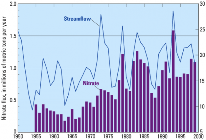
Previous research established a connection between runoff from agricultural operations in the mid-continent region into the Mississippi River drainage and development of hypoxia. Wet years (Fig. 9 corresponds to higher flow rates for the Mississippi River and greater delivery of dissolved nitrogen to the coastal region. Note that 1987-89 were years of low nitrate flux (Fig. 9), which correspond to low area of Gulf of Mexico hypoxia.
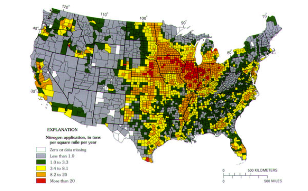
It is also clear from Figure 10 that very high rates of fertilizer application characterize the Mississippi River Basin. Think back to the section called Contaminant Example: Arsenic in Groundwater when you examined nitrate concentration variation in Iowa streams at present. It should be apparent that fertilizer applications and runoff are the main culprits in hypoxia in the Gulf of Mexico.
Module 8: Cities in Peril: Dealing With Water Scarcity
Module 8: Cities in Peril: Dealing With Water ScarcityOverview
In this module, which extends over two weeks, we will explore issues related to water use and scarcity. Major population centers and their burgeoning water needs, particularly those cities located in arid or semiarid regions with sparse local water supplies—Las Vegas, NV, and Los Angeles, CA come to mind as glaring examples. In both of these cases, the main source of water is surface water from distant sources, and we must examine the provisions and history of the Colorado River Compact to understand how water is allocated in the southwestern U.S. Later in this module, we will see how climate change can affect the Colorado River resource. New York City, on the other hand, is located in a region replete with surface and groundwater resources; but the NYC story is of interest because of the incredible planning and engineering that has gone into—and continues— assuring a steady water supply.
But cities are not the main consumers of water, as we have learned. We must also consider the impact of agriculture on water resources; in the U.S. this is, perhaps, best exemplified by the impacts on the huge multistate Ogallala Aquifer system of the Midwest, which has experienced considerable overdraft, primarily as the result of water withdrawals for crop irrigation. This will also serve as one of our water supply foci in this module.
We will also briefly examine how water is regulated. We have, of course, already covered (Module 7) regulation of drinking water quality, but it is equally important to understand who controls water allocations and how. Water resource allocations are much more complicated, with regional variations in water law and the additional impacts of regional and international compacts. Yes, there have been water "wars" (disputes) related to these laws/doctrines/principles, but we will not cover those here to any extent.
In this module our approach will differ from previous modules in that we will provide some background information on the major topics, including key illustrations, but will ask you to carefully read chapters in "The Big Thirst" (our "textbook", remember that?) and a few other articles, and to compose several short essays in answer to questions in the module.
Module 8.1: Cities in Peril: Dealing with Water Scarcity – History and Current Approaches
Module 8.1: Cities in Peril: Dealing with Water Scarcity – History and Current ApproachesIn this first part of Module 8, we will focus on current strategies for addressing water scarcity. In part, these strategies have arisen within the confines of water laws that have shaped the history of water access and allocation, especially in the American West. After a primer on this legacy that defines the "water allocation landscape", you will learn about the wide-ranging portfolio of approaches utilized by Los Angeles and Las Vegas - cities at the vanguard of creative and modern water management - to hedge against water shortage.
Goals and Objectives
Goals and ObjectivesGoals
- Describe the two-way relationship between water resources and human society
- Explain the distribution and dynamics of water at the surface and in the subsurface of the Earth
- Identify strategies and best practices to decrease water stress and increase water quality
- Thoughtfully evaluate information and policy statements regarding the current and future predicted state of water resources
Learning Objectives
In completing this module, you will:
- Compare land use in areas with contrasting access to fresh water
- Calculate the water needed to support a given population and compare with available resources
- Analyze water supply (scarcity) problems and solutions in the Western US
- Evaluate the policy of annexing water rights from both scientific and ethical perspectives
- Assess the sustainability of water banking as a solution to water scarcity in the event of sustained drought
- Assess the long-term effectiveness and scientific basis of the Colorado River Compact
Surface Water Allocation and Management
Surface Water Allocation and ManagementIn the U.S. there are some differences regionally in how surface water allocations are handled. In large part, these differences arose historically and have been modified and given legal standing.
Riparian Doctrine
Riparian DoctrineThis doctrine has its roots in the Code Napoleon (1804) and English Common Law and has been applied primarily in states east of the Mississippi River. The basic provisions in the early 1800s were that:
- so-called "Riparian water rights" extend to the center of a non-navigable water course;
- navigable water courses belong in the public domain and cannot be obstructed (although it appears that access from privately owned stream banks could be denied);
- mills or milldams could be developed by landowners with stream bank holdings and could be transferred upon sale of property;
- beyond use for millraces, excess water could not be removed and water returned must be equivalent to that removed in quantity and quality; and
- riparian landowners must be compensated for illegal capture of water by others. This last stipulation was interpreted by the U.S. Supreme Court (in 1827) in a way that gave riparian landowners (those with properties bordering a stream) the right to make "reasonable" use of water in a stream. However, they cannot claim ownership of the water, nor can they divert or dam a stream to the detriment of other riparian landowners.
All states (31 states) east of the Mississippi River have water allocation laws based on the Riparian Doctrine. Any waterway that can be used for navigation in its normal condition is considered navigable. If it is only used for intrastate commerce or transport, it is under control of that state. If used for interstate or foreign commerce or transport, it is under the control of the Federal government. There is no "water ownership" under the present Riparian Doctrine and principles of Reasonable Use and Correlative Rights are applied. Riparian landowners can use any quantity of water as long as it does not interfere with the rights of other landowners. They must also, therefore, share the total flow of stream water with other riparian landowners; for example, during a drought, restrictions on water extraction can be enacted to allow all owners (users) a reasonable share of the reduced flow in proportion to their ownership of stream bank property. During floods, riparian landowners can take exceptional action to protect their property, regardless of consequences for other landowners. In addition, the Riparian Doctrine is being altered in some states to allow permits to allocate water based on rates of use and other factors that can be changed by the state at any time. Courts or state water agency officials settle disputes over alleged injurious water use. The Riparian Doctrine works because water resources east of the Mississippi River are not, in general, limiting and irrigation for agriculture is not necessary.
Doctrine of Prior Appropriation
Doctrine of Prior AppropriationThis water law principle developed somewhat gradually in the western U.S. Many western streams had intermittent flows that were not amenable to the specifications of the Riparian Doctrine. Initially, the sparse settlement, general lack of competition for water resources, and seasonality of flow of western rivers allowed landowners to modify river channels to impound water for their use—first-come, first-served. Certainly, the Federal government did not anticipate widespread settlement of the West because it was so arid. By the early to mid-1800s, the influx of Mormon settlers in Utah required some solution to relatively sparse water resources in the face of increased agricultural activity. In response to the need and their religious principles, they established a water allocation system that favored shared use of that resource with a principle that favored beneficial use. However, the beneficial use philosophy was later replaced by that of the "Prior Appropriation Doctrine."
The Prior Appropriation Doctrine grew out of the California gold rush, and the need for gold miners to establish some system of mining claims and water use because of the limited water resources available. This is where the "first come, first served" aspect of water rights arose. California, which became a state in 1850, therefore adopted the Doctrine of Prior Appropriation that allowed diversion of water from a watercourse for use on non-riparian lands. In other words, if irrigation of crops or washing of mine tailings was required on lands with no direct stream access, these uses were permitted, with a priority (time of claim) basis. This doctrine established water rights, based on priority use, that could be sold or transferred as long as they did not interfere with another prior appropriation (" first in time, first in right" as long as this appropriation was properly filed). This doctrine prohibited "junior" (later claimants) users from using water if the resource was so limiting as to reduce that available to "senior" claimants below their allocation. Presently, the "California Doctrine" allows the application of both the Riparian Doctrine and the Doctrine of Prior Appropriation to operate (the so-called California Doctrine), depending on the availability of water resources (e.g., more water-rich northern California vs. arid southern California). Other states had somewhat different histories, but still made use of modified versions of the Doctrine of Prior Appropriation. Colorado, in particular, established the doctrine with respect to agricultural use for non-riparian lands. An interesting aspect of the Prior Appropriation Doctrine is the "use it or lose it" aspect. Once a claim is made, the water use must meet the stipulations of the claim annually, or, potentially, lose that claim. New claims relating to the expansion of irrigation, for example, are treated as "junior" claims that may or may not be honored, depending on the surface-water flow rate and other more senior claims.
Colorado, Alaska, Arizona, Idaho, Montana, Nevada, New Mexico, Utah, and Wyoming presently apply the strict Doctrine of Prior Appropriation as established in Colorado. California, Kansas, Nebraska, North Dakota, Oklahoma, Oregon, South Dakota, Texas, and Washington use the California Doctrine, whereas Hawaii applies its own version of priority depending on the water use.
Activate Your Learning: 2-Minute Essay
Read the question below and write about what you think for just two minutes.
If you raised crops on 100 acres in Pennsylvania and owned land that did not border a watercourse, how might your experience differ from farming 100 acres in Nevada if you did not own land bordering a perennial stream? Set a timer on your cell phone or computer for two minutes.
If you lived in Pennsylvania, you could drill a well to access groundwater to irrigate your crops. In Nevada, this would not be a feasible option. If your land didn't border a stream, you would need to divert water from somewhere else.
Cities in Peril: LA
Cities in Peril: LAThe Giant Straws of Los Angeles
To see Los Angeles, with its lush landscaping and common swimming pools, one would never believe it to be water limited. Los Angeles is a sprawling agglomeration of towns and neighborhoods spread over nearly 470 sq. miles (1220 sq. km) of semiarid hills and valleys (precipitation is about 15 in--38 cm-- annually). One river, the Los Angeles River, runs through the city to the sea, but this watercourse flows only intermittently and--mainly for flood control--has now been straightened and confined to a concrete channel. The City of Los Angeles now has nearly 3.9 million people living within its borders, a far cry from the estimated 1600 people that lived there in 1850 when (a smaller footprint) LA was first incorporated (Fig 1). By 1900, LA's population had grown to over 100,000, and the local water supply was deemed inadequate. Thus began LA's quest for additional water resources. The subsequent history of water acquisition, especially that of Owen's Valley water and the LA aqueduct (see L.A. Aqueduct Centennial 2013 for pics) engineered by William Mulholland, makes very interesting reading ("Cadillac Desert" by Marc Reisner, p. 54-107). Controversy still surrounds this acquisition. Table 1 shows the major aqueducts that now supply water to LA. If you aren't familiar with the term, an aqueduct is an artificial channel for conveying water, typically in the form of a bridge across a valley or other gap.

| Aqueduct | Year Complete | Year Construction | Length | $ Cost | Delivery |
|---|---|---|---|---|---|
| Owens Valley and LA Aq | 1913 | 5 | 223 mi | 23mill | 485 cfs |
| Second LA Aq. | 1970 | 5 | 137 mi | 89mill | 290 cfs |
| Colorado River Aq. | 1941 | 10 | 242 mi | 220mill | 1600 cfs |
| California Aq. and West Br* | 1973 | 1960 appop | 701 mi | 5200mill | 4400 cfs |
*California State Water Project: note that the length and cost is for the entire system, not just LA, and the cfs for the West Branch is not what LA alone receives. Source: California State Water Project At a Glance

The second LA Aqueduct was built to take advantage of additional water taken from the Mono Lake drainage through an 11-mile tunnel drilled under the Mono Craters to connect to the Owens Valley system. Today, about 70% of LA's water comes from the Eastern Sierra. The two LA aqueducts supply nearly 430 million gallons per day (about 100 gpd per person in the City of Los Angeles today!). Groundwater wells in the San Fernando Valley and other local groundwater basins supply 15% of water needs, and purchases from the Metropolitan Water District (Colorado River Water and California State Water Project) supply the remaining 15%. Variation in use of each of these sources year by year (Figure 2) is a function of water supply available at the source resulting from drought, competing uses, and other factors. For example, the period between 1987 and 2004 required the purchase of considerably more water from MWD sources (at greater expense) because of severe drought/low snowpack in the eastern Sierra Nevada during that period.
Activate Your Learning: Think about it!
Imagine if your hometown annexed water rights from somewhere as far away as Mono Lake is from Los Angeles. Where would that water come from for your hypothetical case?
Water Use Trends in LA
Water Use Trends in LA
The trend in total water use for the City of Los Angeles (Figs. 3 and 4) is interesting because, although the population has increased significantly since 1970, average demand has remained relatively constant between 600 and 700 million acre-ft per year and has even decreased to around 500 million acre-feet in the past few years. This is a testimony to the effects of conservation and reuse because of source limitations (competing uses, drought) and rising costs. Economic downturns may also play a role. Certainly, one way to conserve water in LA is through limiting outdoor water use (car washing, landscaping/lawns). It is estimated that watering landscaping for individual homes is about 38% of total water use. Perhaps, like Las Vegas, LA should further encourage xeriscaping and graywater use for irrigating lawns and golf courses, but more on solutions in Module 8, Part 2 next week.

Cities In Peril: Las Vegas
Cities In Peril: Las VegasThe Survival of Las Vegas

It’s hard to think about Las Vegas without images of stereotypical excess: gambling, bachelor(ette) parties, luxurious hotels, swimming pools, golf in the desert, posh fountains, celebrities, major music, and entertainment acts, and famous restaurateurs. On the one hand, it may seem incongruous that Las Vegas and the surrounding Clark County, which receive only 4 inches of rain per year on average and lie within one of the driest regions on Earth (Figure 5) (as discussed in Module 1), are also home to one of the fastest-growing populations in the U.S. (Figure 6; See also the interactive link in the caption below). On the other hand, it may be surprising that Las Vegas is among the most water-conscious cities in the nation, and as discussed below, despite rapid economic and population growth over the past two to three decades the city has managed to live within the limits of its relatively meager allocation of water from the Colorado River, the main water source for the region (see Colorado River Compact).


A Familiar History of Water and Population Growth
A Familiar History of Water and Population GrowthIn the mid-1800s, early settlers named the area "Las Vegas", Spanish for "the meadows", because the Valley, fed by the Las Vegas Springs, was lush, grassy, and green. The springs yielded approximately 5,000 acre-feet of water per year. As you may recall, this is about the amount of water needed today to support 5,000 families of four, or a population totaling around 20,000. With a plentiful natural water supply, Las Vegas became a key stop and hub for the railroads: first the San Pedro, LA, & Salt Lake City Railroad, and later the Union Pacific.
In the early 1900s, private wells drilled into the valley-fill confined aquifer became commonplace to augment the spring flows, as residents tried to turn the valley into productive farmland. Many of the wells were artesian but were left uncapped (Figure 7). By 1912, the 1000 residents of Las Vegas withdrew about 22,000 acre-feet of water per year from the springs and aquifer. By 1930, a combination of several dry years and increasing demand led to overdraft conditions. In the meantime, the Colorado River Compact of 1922 allocated a small amount of Colorado River water to Southern Nevada (see Sidebar: CO River Compact). However, Las Vegas continued to rely principally on groundwater, and aside from some industrial uses, the Colorado allotment went largely unused until the 1940s. (Note that Hoover Dam, the primary infrastructure that allows surface water storage and withdrawal for Clark County, was not completed until 1936.)

With a steadily growing population and water demand, withdrawals greatly exceeded natural recharge and overdraft of the aquifer worsened. In an effort to reduce groundwater extraction, the Las Vegas Valley Water District was created in 1947, in part to begin using the Colorado River allotment. Despite these efforts, by 1960 the valley’s population had swelled to over 110,000, and almost 50,000 acre-feet of water were extracted from the aquifer annually. The natural springs dried up in 1962, and sustained overdraft led the potentiometric surface to drop by a few feet per year on average. The pattern continued through 1971 until the Southern Nevada Water System began delivery of Colorado River water from Lake Mead for municipal supply – 24 years after the water district was created.
With a plentiful supply (300,000 acre-feet per year) of Colorado River Water ready for delivery and distribution, population growth accelerated, reaching almost 700,000 by 1990 (Figure 8), and about 2 million by 2012. Coincident with the shift to water supply from Lake Mead in 1971, dependence on groundwater gradually started to decline (Figure9). As discussed in more detail below, managed (induced) recharge of the groundwater system using surplus Colorado River water was begun on a small scale in the late 1980s; this “banking” of water in wet years or times of surplus is viewed as one strategy to cope with water shortages.


Current Water Use and Sources
Current Water Use and SourcesCurrently, about 90 percent of Southern Nevada’s water comes from Lake Mead (the Colorado River) (Figure 9); the rest comes from groundwater. Because of the very limited natural recharge to the aquifer system, and the fact that no other surface water is available, Las Vegas depends almost exclusively on the Colorado River to sustain its population and economy. The city is essentially at the mercy of the Colorado River. When the Colorado River Compact was signed in 1922, the allotment of 300,000 acre-feet per year was viewed as generous for the sparsely populated state. However, as may sound like a familiar story, with a rapidly growing economy, combined with good weather and apparently plentiful water, population growth rapidly exceeded most projections (see Figure 5).
Of the water delivered by the Southern Nevada Water Authority, it may be surprising to note that most (almost 60%) goes to residential use (Figure 10). Of this, a large fraction is used consumptively for watering lawns. As discussed in detail in The Big Thirst, incentive programs for removal of turf from parks, common areas, and residences is one strategy to reduce water use. Golf courses and resorts, which are often the stereotypical poster children for water “waste” in Las Vegas, use about 14% combined.
The pie chart shown in Figure 10 provides the first blueprint for conservation efforts and potential re-use, by identifying the key water uses in the district. Moreover, there is also a recognition that not all water uses are “equal”: some require clean water (i.e. residential uses, many industrial uses, medical), whereas others do not (golf courses, parks). As a result, reclaimed and partly treated water may be used for many needs. In Las Vegas, water re-use – essentially getting two uses of the same water - is one part of a diverse strategy to maximize the limited allocation of Colorado River water (additional detail on treatment facilities and pricing for reclaimed water are described on the water district’s website.

Figure 10. Municipal water uses in Southern Nevada as of 2022.
Dealing With Water Scarcity: A Diversified Portfolio
Dealing With Water Scarcity: A Diversified PortfolioDue to a decades-long drought in the Colorado River system (see Sidebar: CO River Compact), the water level in Lake Mead has dropped by almost 170 feet since 2000 (Figure11). This corresponds to a decrease from ~25 million acre-feet of stored water to around 10 million acre-feet. If the lake water level drops to 1075 feet (as of June 2022, it is 1043 feet!), a federal shortage would be declared, triggering a reduction in Nevada and Arizona's allocations. In June of 2022, the U.S. Bureau of Reclamation decarded an emergency request for Colorado River states to reduce use by 2-4 million acre-feet within 18 months.To make matters worse, the two intakes in Lake Mead that withdraw water for Las Vegas cannot function if the lake level drops below 1050 feet (intake #1) or 1000 feet (intake #2). With the possibility of continued dry conditions, and because of their near sole dependence on Colorado River water, Las Vegas has developed a multi-pronged strategy to hedge against uncertainty due to future climate change coupled with likely increased demand due to growth and development in Clark County.

Conservation
ConservationAs you have read about in The Big Thirst: Dolphins in the Desert, Las Vegas has been aggressive in water conservation efforts. Part of these efforts focuses on simple reductions in household water use through education, regulation (i.e. watering restrictions), and incentivized removal of water-intensive landscaping. The city has also implemented GPS technology and pressure and acoustic sensors to monitor leaks in their pipelines to limit leaks and thus maintain high efficiency. As a result of these efforts, per capita, water use in Las Vegas has decreased substantially over the past 20 years or so, from over 340 gallons per day to less than 200 gallons (a 40% reduction!) (Figure 12). The SNWA has set a conservation target of 105 gallons per day fro 2035. As a result, Southern Nevada's total annual water use dropped by almost 90000 acre-feet (30 billion gallons) from 2002 to 2012, even as its population grew by 400,000.
Additionally, as noted above, Las Vegas treats wastewater for re-use, especially for applications that (a) don’t require high-quality water, like watering golf courses and parks; and (b) are consumptive. Re-use, incentivized by lower pricing, effectively allows the same water to be used twice, thus making the modest allotment of Colorado River water go further. Indeed, although Southern Nevada’s gross withdrawals from Lake Mead are almost 600,000 acre-feet per year (Figure 9), this is offset by the return of treated water to the Lake such that net withdrawals (consumptive use) remain at the 300,000 acre-feet limit.

New Sources: Tapping Groundwater
New Sources: Tapping GroundwaterDespite a history of overdraft in Las Vegas itself, Southern Nevada has recently turned its eyes back to the underground as an additional water source – but this time in sparsely populated valleys to the North and Northeast of Clark County (Figure13). The rationale for the SNWA’s “Groundwater Development Project” is that groundwater recharge is partly a function of the area over which infiltration occurs, so distributed withdrawals of groundwater from several large valleys fill aquifers outside of Las Vegas may be more sustainable than focused withdrawals from only the local aquifer system. Additionally, the targeted aquifers are in sparsely populated areas, with relatively small water demand.
Nonetheless, as you might imagine, there has been strong opposition to the plan from both environmental groups and ranchers and residents of these valleys, especially when considering past examples of the annexation of water rights for large cities (e.g., Los Angeles and the Owens Valley) and the negative outcomes for the local communities.

Water Banking
Water BankingAs another hedge against water shortage and climate change, the Southern Nevada Water Authority has entered into a series of “Water Banking” agreements with other the Lower Basin Colorado River states, Arizona and California. In these agreements, Nevada pays the other Colorado River water rights holders to store unused water in times of surplus by injecting it into aquifers. Nevada then receives credits for the stored water; if the water is needed, Nevada uses the credits to draw the equivalent water from Lake Mead, and in exchange, the “banker” withdraws the same amount from the aquifer. Although pumping is energy-intensive, groundwater banking does not require the construction of large reservoirs, and the water is not subject to large evaporative losses.
In its water banking agreement with Arizona, the SNWA paid \$100 M initially and began making yearly \$23 M payments in 2009 that will continue indefinitely. The agreement allows the SNWA to withdraw up to 40,000 acre-feet per year. In 2004, SNWA also began a water banking agreement with the Southern California Metropolitan Water District (the water district that serves L.A.) in which some of Nevada’s surplus Colorado River water is stored in an aquifer in Southern California. The agreement allows the SNWA to withdraw up to 30,000 acre-feet per year, provided that they give 6 months notice. Since 1987, Southern Nevada has also been banking its own surplus water – when available - in the valley’s aquifer for later use if needed. In Nevada, about 333,000 acre-feet have been stored through 2022, and in Arizona’s aquifer, the SNWA has stored 614,000 acre-feet of the Colorado River’s water through 2023.
Learning Checkpoint
1) How much is the cost of water banking per acre-foot? Do you think that’s worth it – and how does it compare to the cost of other water resources?
ANSWER:
2) Do you see a problem with the water banking approach to mitigating drought? Do you think it is sustainable in the long-term? Why or why not?
ANSWER:
The Third Straw
The Third StrawIn 2005, faced with the specter of prolonged drought and projected Lake Mead water level declines, the SNWA board of directors approved construction of the so-called “Third Straw”, a new $812 M intake from Lake Mead that would allow Southern Nevada to physically extract water from the lake at water levels as low as 1000 feet above sea level (Figure 14). Construction of the intake involves boring a 23-foot diameter tunnel through 3 miles of rock, with much of its length beneath one of the Earth’s largest man-made reservoirs!
The new intake will intersect the lake at 860 feet above sea level but will share a pumping station with intake #2, so will only be able to operate at water levels of 1000 feet (the same as for intake #2). The primary purpose of the third straw is to maintain overall system capacity if Lake Mead falls below the 1050 ft water level limit for operation of intake #1. It also will access the deepest parts of Lake Mead, where water quality is highest. The initial plan for the third intake included a separate pumping facility but was removed to cut costs. It is always possible that the $200 million pumping station and pipelines could be added in the future, though if the Lake Mead water level were to drop much below 1000 feet, there would be much bigger problems throughout the lower Colorado River basin.

Figure 14 shows the elevation of Lake Mead on the y-axis versus the year on the x-axis including different water conservation projects. The important take home from this figure is that as we near 2022 we see that water levels drop. But as different conservation projects (in green, pink, purple, etc.) grow, the rate at which water levels drop decreases. In the time series, the thick dashed line represents the hypothetical elevation of Lake Mead due without conservation projects, while the solid black line represents the actual water level. Although water level is still dropping as of 2022, conservation efforts play a large role in stabilizing Lake Mead water levels.
The Colorado River Compact
The Colorado River CompactThe Colorado River flows almost 1500 km from its headwaters in Wyoming, Colorado, Utah, and New Mexico, through Nevada, Arizona, and California, before crossing the border to Mexico and flowing to the Gulf of California. It is the lifeblood of the American Southwest, serving almost 30 million people and enabling cities, industry, and irrigation-based agriculture to thrive in one of the direst climates on Earth (see Figure 1 in Module 8.2). The river also provides hydroelectric power that spurred much of the 20th-century development of the Southwestern U.S.
In 1922, these seven western states and the federal government negotiated an agreement, the Colorado River Compact (Figure 15) to allocate water rights on the river. First and foremost the compact partitioned water between Utah, New Mexico, Wyoming, and Colorado (the Upper Basin States) where most of its discharge originates as snowmelt); and Arizona, Nevada, and California (the Lower Basin States), where population growth and water demand were increasing rapidly (Figure 16).
The compact was borne in part out of the Upper Basin States’ unease that water projects and use of the river (e.g., by construction of the planned Hoover Dam) by the Lower Basin States at the time would, if interpreted through the lens of the doctrine of prior appropriations, impact their future claims to water from the river. The compact specifies that the Upper and Lower Basin would each have the rights to 7.5 million acre-feet of water per year. To accomplish this while recognizing that not all years would be the same, the delivery of 7.5 million acre-feet per year to the Lower Basin is evaluated based on a ten-year running average (i.e. the Upper Basin must deliver 75,000,000 acre-feet for any span of ten consecutive years). In fact, the primary purpose of Glen Canyon Dam, unlike Hoover Dam, which generates hydroelectric power and serves as the distributary dam for the Lower Basin States, is to serve as a large “capacitor” in the river system to help ensure that this agreement can be met. Later amendments to the agreement included the 1928 Boulder Canyon Project Act, the 1944 Mexican Water Treaty, and the 1948 Upper Basin Compact. In combination, these amendments spelled out the allocation of water between the individual states, and also allocated 1.5 million acre-feet for Mexico (Table 1).
Of course, the specification of an absolute amount of water to each of the states and Mexico has raised a few serious problems that remain contentious. First, the river is over-allocated. The 1920’s – coincidentally the time that the Compact was negotiated was an anomalously wet period with annual flows as high as ~20 million acre-feet (Figures17-18). In contrast, the long-term mean discharge of the river is about 15 million acre-feet, yet 16.5 million are allocated. Furthermore, the river flow is highly variable and based on historical data and tree ring reconstructions, it seems that decades-long dry periods with flows less than 13-14 million acre-feet may be common. Second, climate projections indicate that the region will become drier in the long-term, and some have suggested that we have already entered an era of steadily declining river flows along the Colorado. Fourth, improved understanding and renewed interest in the environmental impact of decades of dramatically reduced flow have spurred new pressures to allocate some discharge for the natural system. Finally, demand is likely to increase as populations in the region continue to grow, further stressing the already over-allocated river (Figure 18).


Colorado River Allocations (Million Acre-Feet per year, ten-year running average)
| Colorado | 3.9 |
|---|---|
| Utah | 1.7 |
| Wyoming | 1.0 |
| New Mexico | 0.85 |
| Nevada | .30 |
|---|---|
| Arizona | 2.85 |
| California | 4.4 |
| Mexico | 1.5 |
|---|---|
| Total | 16.5 |
Total of Colorado River Allocations(in Million Acre-Feet per year) = 16.5


Summary and Final Tasks
Summary and Final TasksSummary
In the first part of Module 8, you’ve learned about the water appropriation laws that have shaped access to water in much of the U.S. As you’ve seen, cities, especially in the arid American West, now must operate within the limits of these water appropriations, regardless of population or economic growth they have accommodated in recent decades. The tension between finite water allocation (i.e. from the CO River) and continued growth has motivated a diverse portfolio of strategies in place to cope with water scarcity and potential shortage. You are now well versed in these approaches, and should be able to describe them, and discuss the costs and benefits of each. In the second part of Module 8 (Module 8.2), we will build upon this knowledge and introduce another risk factor for water supply - that of climate change.
Reminder - Complete all of the Module 8.1 tasks!
You have reached the end of Module 8.1! Double-check the to-do list on the Module 8.1 Roadmap to make sure you have completed all of the activities listed there before you begin Module 8.2.
References
Fishman, C. (2011). The big thirst: The secret life and turbulent future of water. Free Press.
Southern Nevada Water Authority. (2024). 2024–2029 joint water conservation plan.
Module 8.2: Cities in Peril: Future Climate Change, Population Growth, and Water Issues
Module 8.2: Cities in Peril: Future Climate Change, Population Growth, and Water IssuesIntroduction
As has been discussed throughout this course, the relationship between humans and water resources has a long and complicated history. Water has played a central role in how and where human civilizations have developed. Proximity to high quality, reliable water sources provides a firm foundation for a thriving society. Societies that have established near unreliable or unpredictable water sources that may dry up during droughts and/or flood unexpectedly and uncontrollably) have struggled and occasionally suffered catastrophic losses. In other cases, societies have suffered more chronic problems with water quality. Advances in engineering have greatly improved accessibility and reliability of water resources, to an extent that is difficult to overstate. In some cases, however, a combination of highly effective engineering and risky (or ill-informed) decision-making has created some sketchy and unsustainable situations, as discussed in the first half of this module. What does the future hold? How, when and where might the legacy of our past decisions cause us severe problems in the future? What new problems might we anticipate as a result of climate change and population growth? Will technology save us? Or will more ecosystem-focused planning provide a more resilient water future for humans? How much of Earth’s water should humans feel entitled to? How much should be left for nature? These are some of the questions we’ll address in part 2 of this module.
Goals and Objectives
Goals and ObjectivesGoals
- Describe the two-way relationship between water resources and human society
- Thoughtfully evaluate information and policy statements regarding the current and future predicted state of water resources
- Communicate scientific information in terms that can be understood by the general public
- Predict how human interaction with water on Earth is expected to change over the next 50 years
- Interpret graphical representations of scientific data
Learning Objectives
In completing this module, you will:
- Argue one of the many viewpoints on climate change.
- Identify the causes of global warming and climate change over the past ~250 years, including anthropogenic and natural influences.
- Assess whether mathematical models are a sound basis for making policy decisions.
- Evaluate the implications of climate change on future water resources for specific locations in the US.
- Devise a water plan for Phoenix, AZ, projecting forward from 1915
Water Use, Water Stress, and Population Growth
Water Use, Water Stress, and Population GrowthModule 1 discussed the who, how and where of water use throughout the US and the world. In the US and most industrialized countries, the dominant water uses are industry and agriculture. Domestic and municipal water use typically comprises only 15-30% of water use. In developing countries, per capita, water use tends to be lower in general, with a smaller proportion dedicated to industrial use and a larger proportion dedicated to domestic uses (see Module 1, Figures 8 and 9).
It is also useful to remember that we don’t actually see most of the water needed to sustain our daily activities. In the US, average per capita ‘direct’ use of water (domestic or municipal, for watering your yard, taking a shower, flushing the toilet, etc.) is 156 gallons per day, but the per capita ‘indirect’ use of water (including water used for energy production, manufacturing, food production, etc.) is 1230 gallons per day. So we really only ever see about 12% of the water that is used to sustain our quality of life. This ‘invisibility’ (as Charles Fishman refers to it in “The Big Thirst”) of our dependency on clean, reliable water is one of the challenges in planning for the future. Often we’re not even aware of what we stand to lose!
Population growth was also discussed in Module 1. The population is expected to grow by nearly a third of what it is today, to around 9.7 billion by 2050.For an engaging look at population increase in real-time, see the US Census Bureau Population Clock. It is all the more concerning that some of the most rapid population growth in the world (India and Africa) is expected to occur in places that are already experiencing water stress. Add to this the legacies of past policies and infrastructure as well as future projections of climate change and it seems that we have a lot of work and planning to do!
Climate Change
Climate ChangeWhat do and don’t we know about climate change?
Global warming and climate change: Both of these phrases have been used, often interchangeably, to discuss what is currently happening to our climate system. The term ‘global warming’ was coined by a Columbia University geochemist and climatologist by the name of Wallace ‘Wally’ Broecker in a 1975 Science article entitled “Climatic Change: Are we on the brink of a pronounced global warming?” Global warming, in the strict definition, refers to the observation that Earth’s average surface temperature is rising due to increased levels of greenhouse gases. The term ‘climate change’ includes global warming, but also considers the myriad other changes to Earth’s climate system that are caused by rising temperatures, including changes in precipitation and evaporation, movement of air currents (be they frontal systems or convective systems, hurricanes or a polar vortex), etc..
There is virtually no disagreement among climate scientists that both global warming and climate change are happening and is primarily due to human emissions of greenhouse gases. Broad agreement on these points among the science community is not because scientists tend to be an agreeable group. To the contrary, scientists are typically quite quick to disagree with one another and discuss their disagreements ad nauseam, in great detail and based on all available evidence, from empirical observations or theoretical physics and chemistry. Scientists also have large incentives to prove one another wrong. If, for example, a scientist was able to provide compelling evidence that increased greenhouse gases are not causing a systematic change in Earth’s climate system (or that evolution is not the driver of biodiversity, or that the Earth is not 4.6 billion years old), he or she would be famous as the likes of Galileo, Darwin or Einstein (all of whom toppled earlier scientific understanding), their work would be well funded (we would consequently have a lot of new questions that would need to be answered!), their book would be a best-seller, they would probably pick up a Nobel Prize and most notably, they would be interviewed by all of the most reputable talk show hosts. But no scientist has made such a compelling case. To the contrary, the case for significant climate change is compelling in both the empirical observations as well as the theoretical predictions. Those who proffer the opinion that climate change is not happening or is a hoax presumably do so out of sheer ignorance and/or because they have a financial incentive to believe (or to have others believe) that to be the case.
Distinct from the question of whether or not climate change is occurring, many questions remain regarding the effects of climate change on societies and economies. Certainly, there are positive effects. Warmer temperatures and increased carbon dioxide levels mean increased plant and crop productivity. Some places are expected to receive increased amounts of precipitation, potentially relieving water stress (though perhaps also increasing flood risk). Other places will most certainly not be so lucky and generally speaking, the risks and expected losses associated with climate change are expected to far outweigh the benefits. A comprehensive review of climate science and climate change is not possible within the scope of this course, but we will review a few of the key points as they relate to water, science, and society. We refer students to the most recent reports from the Intergovernmental Panel on Climate Change for more detailed and updated information.
Who Does Climate Science?
Who Does Climate Science?Just about anyone could do climate science. Agencies, particularly in the US and Europe, have made an immense amount of weather and climate data available and with a modest amount of training and software anyone could perform rudimentary analyses of temperature or precipitation trends (e.g., see ncdc.noaa.gov or weather.gov or prism.oregonstate.edu). Of course, such analyses don’t answer all the questions. Tens of thousands of highly trained, independent scientists around the world collect and analyze climate data and develop models of global or regional climate change, which are typically tested using historical data and projected into the future. To provide a forum for discussion and debate that could be synthesized to represent our best understanding of climate change, the United Nations Environment Program (UNEP) and the World Meteorological Organization (WMO) established the Intergovernmental Panel on Climate Change (IPCC) in 1988. Thousands of scientists contribute data, analyses, and model results to the IPCC and provide critical peer review of any climate-related research, all on a volunteer basis. Six major assessment reports have been generated by IPCC, with the most recent report released in 2023.
What is Causing Global Warming?
What is Causing Global Warming?While it is not our intent in this module to explore this question in detail, it is worth pointing out that many human activities clearly affect the climate system. Most notably, emissions of greenhouse gases, especially carbon dioxide and methane, are causing more heat to be trapped within Earth’s atmosphere. This effect, called the greenhouse effect, has been well understood since it was discovered by Svante Arrhenius in 1896. Figure 1 below, taken from the 2023 IPCC Working Group 1 Technical Summary shows the relative amount of heating or cooling of the climate system that can be attributed to the various factors that have changed between 1750 and 2019. The anthropogenic modifications to the climate system, enumerated in panel (a) of the figure, show the breakdown of radiative forcing. Anthropogenic forcing greatly outweighs the changes due to natural changes in solar irradiance. Panel (b) shows the effect each emitted component has on global surface temperature. The IPCC is quite careful to note the level of confidence associated with any given piece of knowledge, seen here with the black error bars of 5-95%. They are also transparent and are quick to point out when new understanding has significantly changed estimates or predictions, as has happened with our understanding of stratospheric water vapor, which was thought to be a significant contributor to warming in the Fourth IPCC Assessment Report (AR4, released in 2007), but has been found to be less significant.

Learning Checkpoint
According to Figure 1 above, total warming (i.e., positive radiative forcing) caused by human activities between 1750 and 2019 is equivalent to about:
(a) 0 W/m2
(b) 1 W/m2
(c) 2 W/m2
(d) 3 W/m2
(e)This cannot be determined from the graph.
ANSWER: (c) 2 W/m2
According to Figure 1, total warming (i.e., positive radiative forcing) caused by natural processes between 1750 and 2019 is equivalent to about:
(a) 1º C
(b) 1.5º C
(c) .5º C
(d) .25º W/m2
(e)This cannot be determined from the graph.
ANSWER: (a) 1º C
According to Figure 1, total warming (i.e., positive radiative forcing) caused by natural processes between 1750 and 2011 is equivalent to about:
According to Figure 1, the single biggest anthropogenic contributor to global warming is:
(a) Carbon dioxide
(b) Changes in surface albedo
(c) Aerosol emissions
(d) Methane
ANSWER: (a) Carbon dioxide
According to Figure 1, the biggest anthropogenic contributor to global cooling is:
(a) Greenhouse gas emissions
(b) Changes in surface albedo
(c) Aerosol emissions
(d) Tropospheric ozone emissions
ANSWER: (c) Aerosol emissions
What Are the Implications of Global Warming for Precipitation and Water Availability?
What Are the Implications of Global Warming for Precipitation and Water Availability?So what does all this human-induced warming mean for the water cycle and water availability? Thinking back to module 2, you learned that warmer air can hold more water (i.e., warmer air has a higher saturation vapor pressure). Therefore it is reasonable to expect higher amounts of water vapor in the air. This is supported by observations that show a 3.5% increase in water vapor in the past 40 years as the climate has warmed about 0.5°C, with relative humidity remaining approximately constant.
Changes in precipitation are harder to measure (or predict) compared with changes in atmospheric water vapor content because of the immense temporal and spatial variability of precipitation. Nevertheless, patterns of precipitation change can readily be observed from historical records (Figure 2), with many areas seeing increases greater than 25 mm/year per decade (i.e., going from 300 mm/yr to 325 mm/yr over the course of a decade) and other places (particularly Africa and Southeast Asia) seeing decreases in precipitation at rates greater than 10 to 25 mm/year per decade. With increasing temperatures, it naturally follows that a greater proportion of precipitation would fall as rain, rather than snow, which has also been documented by the IPCC.

Learning Checkpoint
According to Figure 2, the two models (CRU and GPCC) indicate that, on average, precipitation throughout the conterminous US has ___________ from 1901 to 2019 (see left column of maps).
(a) increased
(b) decreased
(c) remained about the same
ANSWER: (a) increased
According to Figure 2, all three models indicate that, on average, precipitation throughout the conterminous US has ___________ from 1951 to 2019 (see right column of maps).
(a) increased in some areas and decreased in others
(b) decreased everywhere
(c) remained about the same
ANSWER: (a) increased in some areas and decreades in others. Note that the western US is seeing more dry conditions, and the eastern US is seeing more wet conditions.
Historical Precipitation Records and Climate Models
Historical Precipitation Records and Climate ModelsWhat can the historical precipitation records and climate models tell us about the future?
But what can the historical precipitation records and climate models tell us about the future? Simulating future changes in precipitation patterns is one of the most difficult elements of climate modeling because precipitation and evaporation (there are feedbacks between the two so you have to model both) are driven by complex, non-linear processes. So climate models do not attempt to predict detailed representations of precipitation for any given location and climate models are generally not capable of predicting changes in precipitation intensity or frequency of extreme events, other than the likely sign (+ or -) of expected change. Nevertheless, all global climate models attempt to capture general trends in precipitation and considerable agreement exists among all the many competing models. In the broadest perspective, the IPCC makes the following important projections:
“Changes in the global water cycle in response to the warming over the 21st century will not be uniform. The contrast in precipitation between wet and dry regions and between wet and dry seasons will increase, although there may be regional exceptions.”
“Extreme precipitation events over most of the mid-latitude land masses and over wet tropical regions will very likely become more intense and more frequent by the end of this century, as global mean surface temperature increases (see Table SPM.1).”
“Globally, it is likely that the area encompassed by monsoon systems will increase over the 21st century. While monsoon winds are likely to weaken, monsoon precipitation is likely to intensify due to the increase in atmospheric moisture. Monsoon onset dates are likely to become earlier or not to change much. Monsoon retreat dates will likely be delayed, resulting in lengthening of the monsoon season in many regions.”
“There is high confidence that the El Niño-Southern Oscillation (ENSO) will remain the dominant mode of inter-annual variability in the tropical Pacific, with global effects in the 21st century. Due to the increase in moisture availability, ENSO related precipitation variability on regional scales will likely intensify. Natural variations of the amplitude and spatial pattern of ENSO are large and thus confidence in any specific projected change in ENSO and related regional phenomena for the 21st century remains low.”
Figure 3 shows the average temperature and precipitation results of many different competing models for two different scenarios, comparing observations in 1995-2014 to the projected time period 2081-2100. The figures are aggregates of a number of competing climate models from CMIP6. The two scenarios, called ‘Shared Socio-economic Pathways’ (SSPs) 2.6 and 8.5 are the two end-members of greenhouse gas emissions, with SSP 2.6 assuming that greenhouse gas emissions peak in 2010-2020 time period and decrease aggressively thereafter and RCP 8.5 assuming that greenhouse gas emissions increase throughout the 21st century. Notice that the warming (top plots) is not uniform throughout the world. The higher latitudes, especially in the northern hemisphere are expected to heat up considerably more than the temperate or tropical latitudes. We often hear numbers of the global average increase in temperature (estimated 1-2°C or 2-3.5°F by 2050), but this average value does not represent what is expected to happen at high latitudes. A 3-4°C (5-7°F) increase in the arctic, as indicated by SSP 2.6, represents a dramatic transformation of this ecosystem. A 8-10°C (18-21°F) increase in the arctic, as indicated by SSP 8.5, would represent a complete transformation of this ecosystem. What do you think would be the potential benefits and damages caused by such a transformation?
Changes in precipitation are also not expected to be uniform. In general, increases or decreases in precipitation are expected to be more drastic in the high greenhouse gas emission scenario (SSP 8.5) with some areas receiving 30-40% changes relative to 1995-2014. What ecosystem, economic or social changes might you expect to see as a result of a 30-40% increase or decrease in precipitation in the arctic? In Spain? In South Africa? In Chile?
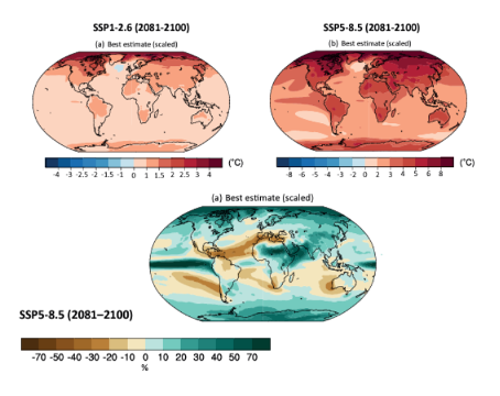
Figure 3. (IPCC chapter 4 figures 4.41 and 4.42) Maps of CMIP6 multi-model mean results for scenario SSP1-2.6 and SSP5-8.5 for temperature and SSP5-8.5 for precipitation. Changes shown from 2081-2100 relative to 1995-2014 averages. IPCC.
Projected Changes
Projected ChangesFigure 4 illustrates projected changes in other parts of the hydrological cycle during the time period 2081-2100 relative to 1986-2005 according to the high greenhouse gas emissions scenario (RCP 8.5). Note that the number of competing climate models represented for each panel of the figure is indicated by a number in the top right (range: 32-39 different models are averaged for each prediction). Future projections of water runoff or soil moisture are dependent on precipitation, which, as discussed earlier, is itself subject to substantial uncertainties. Nevertheless, it is worth considering what the variety of competing climate models have to say. For example, note the general (if slight) decrease in relative humidity over most land masses and a slight increase in relative humidity over the oceans (middle panel, left column). The middle panel in the right column shows changes in the difference between evaporation and precipitation with blue colors indicating a relatively wetter future (more precipitation relative to evaporation) and red colors indicating a relatively drier future (more evaporation than precipitation). The bottom panel in the left column predicts changes in surface water runoff. Note the significant declines in runoff throughout the southwestern US and southern Europe/northern Africa and parts of South America. This same trend is amplified in predictions of soil moisture, which is a primary control on plant growth (bottom panel, right column).
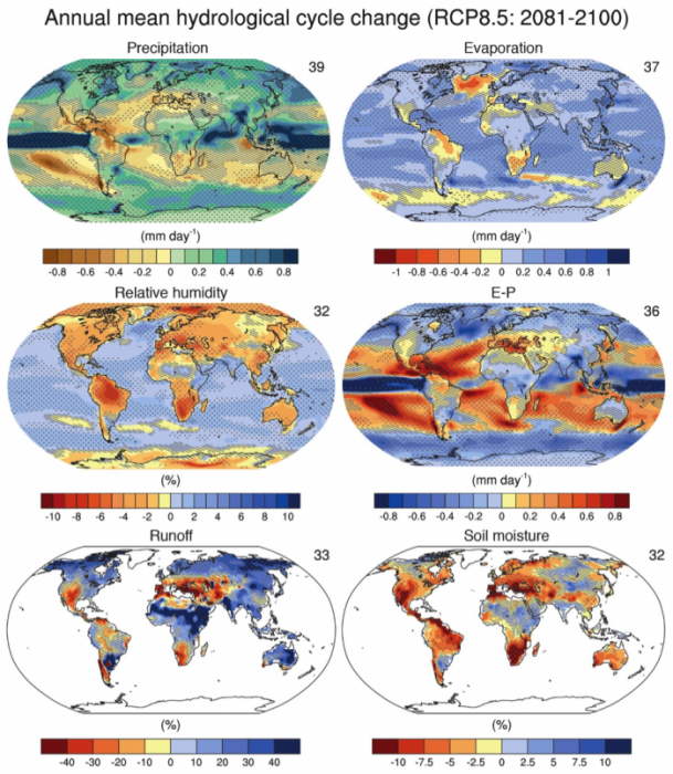
Figure 4. (IPCC TFE.1, Figure 3) Annual mean changes in precipitation (P), evaporation (E), relative humidity, E – P, runoff and soil moisture for 2081–2100 relative to 1986–2005 under the Representative Concentration Pathway RCP8.5 (see Box TS.6). The number of Coupled Model Intercomparison Project Phase 5 (CMIP5) models to calculate the multi-model mean is indicated in the upper right corner of each panel. Hatching indicates regions where the multi-model mean change is less than one standard deviation of internal variability. Stippling indicates regions where the multi-model mean change is greater than two standard deviations of internal variability and where 90% of models agree on the sign of change (see Box 12.1).
All Water Problems Are Local
All Water Problems Are LocalIt is useful to know how climate change is likely to impact the water cycle at the global scale and IPCC reports represent our best understanding of those impacts over the next few decades to a century. But as we have discussed elsewhere, all water problems are local. In very few situations is it even feasible, let alone prudent, to transfer water long distances. Every place has its own set of challenges, institutional and infrastructure legacies, financial or other resource constraints, and concepts of social acceptability.
Generally speaking, places currently experiencing water stress or expecting to experience water stress in the foreseeable future have only a few basic options: a) have fewer people, b) force/incentivize people to use less water, c) increase storage and/or minimize losses within the system, d) reuse water, or e) get water from elsewhere. The capacity to cope with water stress (short or long-term) generally increases with wealth, though in wealthier countries more infrastructure is potentially at risk. As major population centers have already begun to struggle with water shortages it has become clear that massive investments in water technology and security infrastructure can allow wealthy nations to offset higher levels of water stress without remedying their underlying causes. Less wealthy nations, on the other hand, remain vulnerable and have fewer options in water development.
Salt Lake City
Salt Lake CitySalt Lake City: A case study in water development history and planning for the future
Salt Lake City (SLC) provides an interesting case study in terms of the history and future of water resource development. The first permanent settlers of Salt Lake Valley arrived in 1847 and immediately began diverting water from City Creek (northernmost of the four watersheds highlighted in blue in Figure 5). It is estimated that the early settlers hand-dug 1000 miles of ditches in the first few decades to distribute the water to agricultural fields, Salt Lake City and nearby settlements. By 1879 the population of Salt Lake County had grown to nearly 32,000 and the city authorized construction of the Jordan and Salt Lake City Canal, which was completed in 1882 with a capacity of 150 cubic feet per second, expected to provide enough water for 100,000 residents. The canal is still in use today. Several major dams were constructed as early as 1892 to 1907. Following a major water shortage in 1924, Mayor John Bowman proclaimed that ‘a city can never be greater than its water supply’ and initiated an ambitious water development program to supply reliable water for more than 400,000 residents. Several other large dams were constructed from the 1940s to as late as the 1990s to keep ahead of the rapidly growing population, but options for additional water storage via new reservoirs are now very limited.
Today Salt Lake City’s water supply is derived from several mountainous watersheds to the east of the city, in the Wasatch Front and western Uinta Mountains (Figure 5). About 50-60% of the water is derived from the four creeks just to the east of SLC (highlighted in blue), with the remaining portion delivered from the Weber, Provo, and Duchesne rivers via inter-basin transfers (tunnels, canals, and aqueducts shown as blue and white dashed lines in Figure 5) and extracted from groundwater. Around 70-80% of Salt Lake City’s water supply originates as snowmelt. Thus, the storage of water as snowpack, the timing of snowmelt, and water storage capacity within the system are all critical to ensuring reliable water supply.
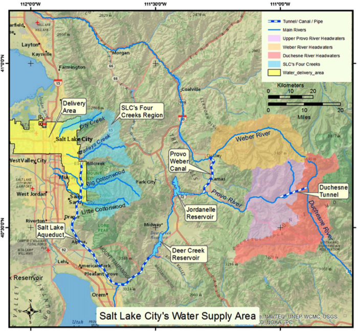
Public utilities water use has remained relatively steady at 80,000 acre-feet of water per year since 1980. To put that number in perspective, imagine a tank of water an acre at its base and 80,000 feet (15 miles) tall, or the equivalent of a tank the size of Central Park in New York City flooded 100 feet deep. The fact that total public water use has remained steady over the past three decades is an impressive feat considering the population of Salt Lake County has nearly doubled from 620,000 in 1980 to nearly 1.1 million in 2014. Much of the Greater SLC area is populated by members of the Mormon religion, which has traditionally emphasized large families. More recently the size of families has decreased, but the population as a whole continues to grow.
Despite a growing population, total water use has started to decline in the past decade despite the fact that this time period includes three of the hottest summers on record, due to effective public education and water conservation campaigns (Figure 6).

Climate Change Further Complicates the Water Situation
Climate Change Further Complicates the Water SituationClimate change further complicates Salt Lake City’s water situation. Peak supply from the four creeks typically occurs in early June and is expected to shift earlier in the year, to mid-May, in the coming decades. However, peak water demand typically does not occur until late July or early August. Hence the need for significant amounts of water storage. Temperature increases over the past few decades have already resulted in more winter precipitation falling as rain, rather than snow, thus reducing snowpack. The increased proportion of precipitation falling as rain, combined with an earlier snowmelt threaten the system’s ability to maintain adequate water supply through late summer. The total amount of water runoff is also expected to decrease as the climate warms. Every degree Fahrenheit of warming in the Salt Lake City region could mean a 1.8 to 6.5% drop in the annual flow of rivers that provide the city’s water supply. The semi-arid region is also known to experience frequent and sometimes prolonged drought. With a growing disparity in the timing and potentially the volume of water supply/demand, clearly, some changes are needed. Options currently being considered are further reductions in demand, additional water storage within the system, or extraction of groundwater.
Unfortunately, groundwater reserves are not in great shape. The shallow, unconfined aquifer underlying much of the valley is contaminated from uranium mine leachate, chloride, sulfate, iron, uranium, volatile organic compounds, and pesticides. Recent water quality testing from the shallow, unconfined aquifer found all samples to be below acceptable standards for drinking water. There is a deeper, confined aquifer that is in much better shape, with more than 80% of water meeting or exceeding water quality standards. However, excessive pumping of this aquifer has drawn down the water level by as much as 30-50 feet in places, from 2000-2022.
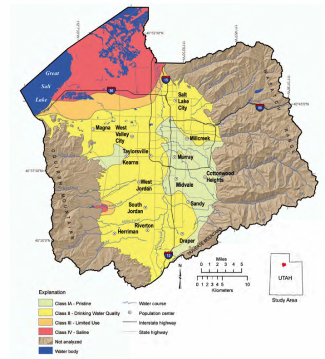
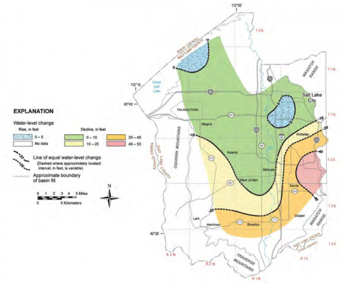
With the Great Salt Lake immediately adjacent to the city it might seem like desalination might be an option. Desalination, also called desalinization, is the process of removal of salt and other minerals to produce fresh water for consumption or irrigation. This is most commonly achieved by boiling water in a process called vacuum distillation or a process called reverse osmosis in which water is forced through a permeable membrane that strips out the salts. Either approach requires a considerable amount of energy and is therefore typically more expensive than most any other alternative. Considering that the Great Salt Lake is 3-8 times more saline than the ocean, this solution is currently not economically feasible to do on a large scale, though some desalination is currently done to treat partially saline groundwater.
People are, of course, not the only organisms that require access to clean and reliable freshwater. More than 75% of the wetlands in the state of Utah are found in Salt Lake Valley, which contains a wide variety of plant species, play an important role in regulating water quality, and provide habitat for a variety of birds, amphibians, and other animals. In addition, several threatened and endangered fish and bird species are dependent on the perennial flowing streams and rivers in the area. Water-stressed trees within the urban forest of the Greater SLC area have become more susceptible to disease. Lower precipitation in the mountains has increased the number and severity of wildfires.
Led by Mayor Ralph Becker, Salt Lake City has taken a proactive stance to adapt water resource management practices and mitigate the effects of climate change. Mitigation involves reducing the magnitude of the problem itself, whereas adaptation involves limiting one’s vulnerability to expected impacts. As part of the Water Conservation Master Plan, the city is attacking the problem from multiple angles. As a preventative measure, the city is purchasing and protecting large tracts of land in the watersheds that provide drinking water. SLC is also incorporating future climate scenarios into city and water development planning efforts, which is quite progressive for a state whose legislature passed a resolution in 2010 proclaiming that climate change was essentially a hoax.
The city is also attempting to bolster local resilience and reduce dependency on external sources of food, recently having passed several ordinances that promote local food production and community gardens. Also, the city is developing a water re-use program to provide water for city parks, golf courses, and the urban forest.
Recognizing that energy demand is a large and growing water use sector, the city is providing incentives for individuals and businesses to minimize the use of all forms of energy and invest in energy-efficient upgrades. Incentives are also in place for the use of solar energy (photovoltaic cells) and solar hot water heaters. The city has promoted net-zero building approaches (meaning that the amount of energy used by the building on an annual basis is roughly equal to the amount of renewable energy created on-site). And they have been willing to put their money where their mouth is…SLC’s Public Safety Building, completed in July 2013, is the first public safety building in the nation to be designed as a net-zero building and one of the first to meet the US Green Building Council’s LEED Platinum certification criteria. Climate change scenarios are being considered in many aspects of infrastructure planning, including building roads and sewers to handle higher runoff volumes and warmer temperatures. In recognition of the progressive direction, he has taken Salt Lake City Mayor Becker was appointed to President Obama’s climate adaptation task force in November 2013.
Module 9: Water and Politics
Module 9: Water and PoliticsOverview
We have introduced some of the science and society issues in the first eight modules, and you have, by now, soaked up what you need to know to begin to formulate your own strong impressions of the major local and global issues and to come to some conclusions regarding possible solutions to them. In modules 9 and 10, we will expect more of you in the way of synthesis and solution.
The Pacific Institute has compiled a very cool, comprehensive list of water conflicts (Pacific Institute: The World's Water) spanning recorded human history. Each event is accompanied by a brief account of the issue. Many of the earlier events chronicle the attempts to use water as an instrument of warfare—as a barrier to invasion, poisoning of water wells to deprive enemies of water, or destruction of water impoundments and irrigation systems, for example. World politics and creation of new nation-states in the twentieth century, however, created a different sort of conflict based on the need to divide crucial water resources between developing countries with burgeoning populations.
In this module, we will entertain several examples of international "water wars," referring to conflicts that occur within or between countries as the result of failed treaties and agreements, water supply interruptions, climate- or population growth-induced water shortages, and related issues. You are already familiar with an early and ongoing water conflict that involved the California-based antagonism between the City of Los Angeles and the Owens Valley beginning in the early 1900s (a conflict briefly entertained in Module 8.1 and related activities). Such episodes have a familiar cause—population growth, growing water shortage, acquisition of water, conflict, growth stimulated or supported by new water resources—creating a vicious cycle, as in the Los Angeles case.
Chapter 7 in "The Big Thirst" deals with the effects of climate change on rainfall in areas of already limited rain in Australia and suggests that this may be a problem for the long term. So-called "cli-fi," films, with apocalyptic climate-change scenarios at the heart of their plots, have become popular. No less than the Office of the Director of National Intelligence, which oversees all American intelligence agencies has released a report that suggests that climate change, and its influence on water availability, is a major near-future security issue. The United Nations World Food Program has estimated that 650 million people are living in areas where flood and drought can lead to food shortages and price spikes. For example, in East Africa, drought has led to warring among Somali clans for access to potable water. You should keep in mind the lessons of Module 8 Part 2 as we examine water "sharing" in this module—climate change enters into consideration of all of the examples herein, but is only explicitly mentioned in section called "The United States and Mexico—Sharing the Flow?" for the Colorado and Rio Grande River systems. A good example of internal issues related to recent climate change (prolonged drought) and poor government policy can be found here for Iran Washington Institute.
Goals and Objectives
Goals and ObjectivesGoals
- Describe the two-way relationship between water resources and human society
- Synthesize data and information from multiple reliable sources
- Thoughtfully evaluate information and policy statements regarding the current and future predicted state of water resources
Learning Outcomes
In completing this lesson, you will:
- Analyze the political problems that arise when water supplies must be shared across borders
Sharing the Waters
Sharing the WatersThere are many examples of water disputes involving cross-boundary uses of shared resources. Three of these examples will be discussed in this section: The Nile River Conflict, The India-Bangladesh Ganges River Split, and The United States and Mexico— Sharing the Flow.
The Nile River "Conflict"
The Nile River "Conflict"There are many examples of water disputes involving cross-boundary uses of shared resources. For example, in Module 5, we discussed the damming of the Nile River in Egypt and the Nile River's importance to development and water supply in Egypt. The construction of the Aswan Dam, which was authorized by a Nile Waters Agreement of 1959, was of little immediate concern to countries in the source regions of the Nile (Figs. 1 and 2), but guaranteed water rights allocated by earlier agreements were. Egypt initially negotiated the Nile Waters Agreement of 1929 with, what was then, a number of East African colonies of Britain (British as signatories). Through this agreement, Egypt was assigned rights to 48 billion cubic meters/year (bcm/y), including all dry-season flow (mainly from the White Nile), and Sudan, just to Egypt's south, was initially apportioned 4 bcm/y. In addition, Egypt had the right to veto upriver water projects. A later treaty, the so-called 1959 Nile Waters Agreement between Egypt and Sudan, allocated 55.5 bcm/y to Egypt and 18.5 bcm/y to Sudan—the total allocation was nearly 90% of the estimated average annual Nile River flow (84 bcm/y, mostly from the Blue Nile)! This was accomplished prior to independence for the other countries within the watershed and failed to include the monarchy of Ethiopia in negotiations. Interestingly, at the time of the agreement, the White Nile was considered, in error, the source of most of Nile water. Seasonal summer monsoonal rains in the Ethiopian Highlands are the source of much of the Nile waters, through the Blue Nile.

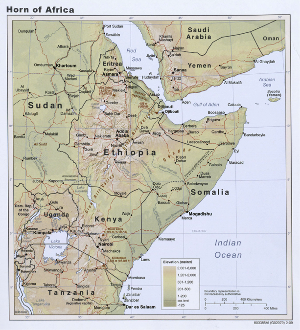
Conflicts have arisen, particularly since Ethiopia embarked on dam building. In 2010, six of the nine upstream countries (Ethiopia, Kenya, Uganda, Rwanda, Burundi, and Tanzania) signed a Cooperative Framework Agreement seeking more water shares from the Nile. Egypt and Sudan rejected the agreement because it challenged their historic water allocations but to no avail. A major dam on the Blue Nile, the Grand Renaissance Dam, is under construction near the Ethiopia-Sudan border. As of May 2016, the dam was about 70% complete, with a target date of 2017 to begin producing power (it is worth noting, however, that the original target date was 2015 - political conflict and construction issues have slowed progress on the dam). Sudan and Egypt are, understandably, concerned about what will occur to Nile flows as the reservoir behind this huge dam fills, but Ethiopia is hoping that the water and power supplied by this structure will boost their economy and help other surrounding nations as well. Ethiopia's population in 1950 was about 18.1 million, but by 2023 it had grown to 126.5 million (114 people/km2). In 1950, Egypt had a population of 21.5 million, and in 2023 there are 112.7 million (112 people/km2).One can see that demand for water must be increasing (source: United Nations Department of Economic and Social Affairs), and that Ethiopia's growth has outstripped that of Egypt. However, Ethiopia has some other sources of water (estimated total river runoff at 122 bcm/y and additional large groundwater resources estimated at 6 bcm), whereas Egypt and Sudan must depend primarily on Nile water. However, Ethiopia has no storage capacity, hence the move to build a number of large dams. Will Egypt and Ethiopia go to war over Nile water? (see Analysis: Why Ethiopia and Egypt aren’t fighting a water war for a perspective ).
The India-Bangladesh Ganges River Split
The India-Bangladesh Ganges River SplitBangladesh achieved independence from Pakistan in 1971, following a short uprising. Bangladesh occupies the region of the original state of Bengal in India, which first became East Pakistan in 1947. India supported Bangladesh in the conflict with Pakistan.
The Ganges River (Fig. 3) was supposed to be shared in some way between India and Pakistan. It is fed by many tributaries (54) the largest of which is the Brahmaputra River that flows through Bangladesh, but most of the Ganges River Basin is in northeastern India. Summer monsoons deliver nearly 80 percent of annual rainfall for this region resulting in peak river flows from June-September. In an average year, it is estimated that 1200 billion m3 of precipitation falls in the Ganges catchment. Of this, nearly 500 billion m3 moves downriver. Dry season flows are much reduced.

India's proposal to construct the Farraka Barrage (a large dam) in West Bengal on the Ganges River right near the border led the two countries to meet over disputed water claims that originated in the 1950s following Bangladesh statehood. There was no resolution to the conflict and the dam was put into place by India without an agreement, with completion in 1975. The dam was constructed to divert some proportion of the Ganges flow into the Hooghly River (during the dry season in order to remove silt that was negatively affecting the port of Calcutta or Kolkata, Fig. 3). Although Bangladesh complained to the United Nations following severe water shortages in 1976, there was no significant resolution until 1996, when India and Bangladesh signed a 30-year treaty that provided for the partitioning of the flow of the Ganges River. The Ganges forms a border between the two countries for part of its course and continues to flow through Bangladesh to the Bay of Bengal. The 1996 treaty guaranteed India a flow of nearly 1000 m3/sec between January 1 and May 31. Much of the time Bangladesh receives less water than allocated by the treaty. India's population in 1950 was 376.3 million while the population of Bangladesh was only 37.9 million. Now India's population is 1.4 billion, (425 people/km2) and the Bangladesh population is 168.7 million (1136 people/km2). Bangladesh has a much greater population density but both countries have a great need for clean water and dependable water supply.
The United States and Mexico—Sharing the Flow?
The United States and Mexico—Sharing the Flow?Most people in the U.S. probably don't think much about what water Mexico takes from the Colorado or the Rio Grande Rivers, which originate in the U.S. and flow along the U.S.-Mexico Border for some distance, and, in the case of the Colorado River, flow through Mexico to the sea (Fig. 4). Like the examples above (the Nile and Ganges Rivers), there are treaties that provide for sharing of the flow of these two North American rivers between the U.S. and Mexico. You have already read about the Colorado River Compact of 1922 (Module 8.1). In effect, the flow of the Colorado River is, on average, significantly less than the total amount apportioned to individual states in the watershed. The 1922 Colorado River Compact was vague about the amount of water that was to be supplied to Mexico. This was rectified in a 1944 Treaty that provided for 1.5 million acre-feet of water per year to flow to Mexico (about 10% of the average Colorado River flow).
The Colorado
The ColoradoUntil the present, the U.S. has bypassed the requisite amount of water from the Colorado to Mexico every year, regardless of the total flow of the Colorado. Because of recent severe droughts in the southwestern U.S., however, a 5-year Agreement (Minute 319), signed in 2012, was brokered that allows the U.S. to reduce the amount of water shared with Mexico when Colorado River flow was much lower than normal. In that agreement, Mexico, which has little Colorado River storage capacity (only Morelos Dam and reservoir), will be allowed to store some of its surplus water in Lake Mead, behind Hoover Dam. In addition, the U.S. will help finance improvements to Mexico's water infrastructure ($21 million), which was badly damaged by an earthquake in 2010, and pledged to "reconnect" the Colorado River with the Gulf of California. The U.S. and Mexico committed to each supply 5,000 acre-feet of water a year to the delta. Accoring to the LA Times in 2014, because of the Agreement, a "pulse flow" event occurred whereby, in March, nearly 105,000 acre-ft of water was released from Morelos Dam (Mexico) to restore (at least briefly) flow to the Colorado River Delta in the Gulf of California (Fig. 5). The intent was to begin to restore riparian ecosystems along the Colorado River in Mexico. However, in 2022, Mexico’s share of water was cut by 5% and nearly 7% in 2023. These pulse flows continue every spring and vegetation is beginning to thrive.

Of interest is the fact that there was more to the water allocation Treaty of 1944. In that Treaty, both the amount and quality of water allocated to Mexico were stipulated. The TDS of waters released to Mexico had to be below 1000 ppm. Alas, the salinity of Colorado River water behind Morelos Dam was typically greater than that because of evaporation and irrigation return flow (leached salt from arid-region agricultural soils in southern Arizona) So, the U.S. built desalinization plant in 1975 near Yuma to treat water to reduce TDS to maintain the agreed-upon values behind Morelos Dam in Mexico (actually partly in Arizona) according to stipulations made by the International Boundary and Waters Commission (IBWC) in 1973. However, the plant was never put into operation because of a period of high flow and lower salinity on the Colorado River. During the period 1973 to 2006, all the return flow from agricultural operations in the Yuma region (TDS=2500ppm; avg. nearly 125,000 acre-ft) was released to Mexico and flowed to the Ciénega de Santa Clara wetlands in Mexico (Fig. 6). This flow substantially contributed to the significant ecological development of the Ciénega as a wetland. In 2011, however, the desalination plant was tested for a year, and the flow of water to the Ciénega de Santa Clara was substantially reduced, with an associated increase in total dissolved solids (TDS>3200ppm). It remains to be seen whether the relatively low treatment volumes (30,000 acre-ft/y) of the desalination plant as configured are a benefit in light of concerns over the fate of the renewed Ciénega de Santa Clara ecosystem (over 30 yrs of runoff) and its endangered species (Yuma Clapper Rail and desert pupfish).
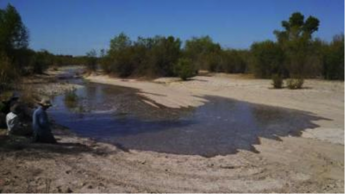
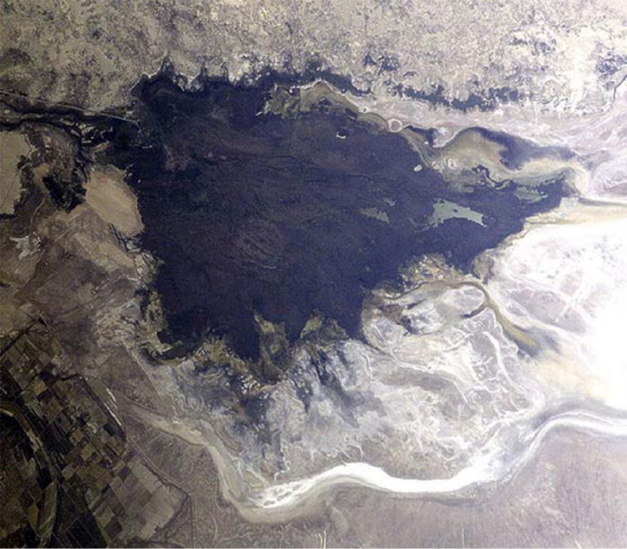
The Rio Grande
The Rio GrandeThe Rio Grande River flows along the U.S. (Texas)-Mexico border for nearly 1,248 miles (2,008 km) including meanders. Although snowmelt from the San Juan Mountains of Colorado (Fig. 7) is a major source of water for the Rio Grande, runoff from northern Mexico also contributes to its flow. As in all arid to semiarid regions, the waters of the Rio Grande River are highly sought after and overallocated. And, as in the case of the Colorado River, the water division between the U.S. and Mexico is regulated by Treaty (see below).
Rio Grande River water is in demand because of the intense agriculture in New Mexico-Texas (Fig. 8) as well as in northern Mexico. This water supply deficit has been exacerbated by prolonged drought in the southwest. Figure 9 is a long-term record of flow of the Rio Grande River (at Otowi Bridge) reconstructed by tree ring records calibrated to more modern flows (see TreeFlow). Note the frequent cycles of surfeit and drought, and the most recent steadily decreasing flow trend beginning about 1990.

In all, there are 15 dams on the Rio Grande River, many of them in New Mexico. Flows are significant until Elephant Butte Reservoir in New Mexico. El Paso, TX is 125 river miles downstream of Elephant Butte Reservoir and just upstream of the American Dam. Releases from Elephant Butte Reservoir control streamflow to El Paso. At American Dam, much of the flow in the Rio Grande is diverted for irrigation and municipal uses in Texas and Mexico. From the American Dam, the Rio Grande has little or no flow until joined by the Río Conchos about 300 miles downriver, which originates in the Sierra Madre Occidental in Mexico (see below). The Pecos River, a major U.S. tributary, joins the Rio Grande another 300 miles or so downriver near Langtry, TX (Fig. 7); the Pecos flow is also controlled by a dam upstream from its confluence with the Rio Grande. Further downriver, the flows in the Rio Grande River decrease significantly as the result of withdrawal for agricultural and municipal use in southwest Texas as well as the relatively low influx of water from tributaries. In Some years, the Rio Grande flow does not even make it to the sea near Brownsville, TX.


About 75% of water withdrawals from the Rio Grande River are in support of agriculture. Population growth has also been a factor, particularly in Mexico, where the population has nearly doubled since 2005, and nearly 6 million people depend on the Rio Grande River and related groundwater basins for drinking water. The U.S.-Mexico Treaty of 1848 established the international boundary, modified slightly by later "Conventions." The Treaty of 1944 between the two countries partitioned water from the Rio Grande River along the Texas-Mexico Border (as well as stipulating Colorado River flows to Mexico, see above), modified slightly by a 1970 Treaty, and authorized both countries to construct, operate, and maintain dams on the main channel of the Rio Grande. The International Boundary and Water Commission (IBWC) was assigned the task of dealing with water quality issues along the international border.
According to the Treaty of 1944, the U.S. is entitled to about one-third of the flow of the Rio Conchos from Mexico, which amounts to about 350,000 acre-ft/y on average. By the Treaty, Mexico is obligated to release 1.5 million acre-ft over a five-year period. During times of drought, it is difficult to meet the annual expectation, and, typically, Mexico releases more water in good rainfall-runoff years and conserves during drought periods, although at one point Mexico did not meet their obligation for nearly ten years. This pattern makes it difficult for agriculture in southwest Texas because water resources cannot be adequately predicted, and, in 2013, a controversy erupted between Texas and Mexico because of long-term drought that peaked in 2011 (Texas Observer: On the Border, a Struggle over Water) --another example of the difficulties of sharing even major rivers.
Systems Thinking: Controls on Rio Grande River Flow to the Sea
Systems Thinking: Controls on Rio Grande River Flow to the SeaConsider the water supplied by the Rio Grande River. In many years there is a trickle of water, or less, that reaches the sea. Why? Obviously, the water inputs are less than or equal to the outputs.
The Rio Grand
Activate Your Learning
Construct a simple system diagram that represents the interplay between the "forces" that influence the flow of the Rio Grande River. Think about aspects of climate, population growth, and water demand as they influence Rio Grande River flow to the sea. Treat the Rio Grande flow/storage as a "reservoir" (total annual water availability in that system) and consider the most important inputs and outputs and the factors that drive them (refer to Module 1 for a background on systems thinking and systems diagrams). When you complete your system diagram on paper, click on the link to see what we expected you to include.
ANSWER:

Once you have studied the diagram, construct the "equations" for Annual Runoff and Annual Water Demand. Do the units match? How do you think this system would behave if the changes in inputs and outputs were large on a yearly basis?
ANSWER:
Annual Runoff= Climate Variation x Annual Precipitation x Drainage Area
Annual Water Demand= Evaporation + (Water Use/Person x Percent Growth/y x Population)
If decreases in Runoff and increases in Water Demand were large (e.g. >1%/year) the Rio Grande would likely not flow to the sea. You could test this by putting realistic numbers into a model using these system relationships and running for several years.
Module 10: Solving the Water Crisis?
Module 10: Solving the Water Crisis?Through the course of the semester and the first 9 modules of the class, you’ve learned about the science of water – including the distribution of fresh water; the demand for water and its relationship to geography, uses, population growth, and climate; and the physical principles that govern surface water and groundwater replenishment and movement. You’ve also considered some of the historical, political, ethical, and economic issues with water allocation and management, for example by considering the impacts of dams, or the annexation of water rights to support cities in arid regions.
In Module 10, the culmination of the course, you will explore potential solutions to the problems of water quantity and quality, especially in the face of population growth, increasing energy and food demands, and greater awareness of (and sensitivity to) the environmental impacts of water development. As major population centers, many of which are not ideally located with respect to water resources, continue to grow, we are faced with serious questions about sustainability: How can water supply and quality be assured, and balanced between the demands of irrigation and cities? Is there a technological panacea, or is a mixed portfolio of approaches required? Is it possible to hedge against climate change and predicted shifts in the timing and spatial distribution of precipitation? How can cost be managed, while minimizing the impact on the environment? Can diverse cultural and political entities work together to implement solutions, or deal with side effects, that cross state, and national boundaries?
Goals and Objectives
Goals and ObjectivesGoals
- Describe the two-way relationship between water resources and human society
- Explain the distribution and dynamics of water at the surface and in the subsurface of the Earth
- Synthesize data and information from multiple reliable sources
- Communicate scientific information in terms that can be understood by the general public
- Identify strategies and best practices to decrease water stress and increase water quality
- Predict how the availability of and demand for water resources is expected to change over the next 50 years
Learning Objectives
By the end of this lesson, you should be able to:
- discuss the costs and benefits of desalination as a solution to water scarcity
- explain the benefits of water re-use
- describe the advantages and disadvantages of water optioning and water banking
- evaluate multiple approaches for safeguarding against water scarcity
- develop a portfolio of strategies for a water-poor urban area
Potential Solutions to Problems with Water Scarcity and Quality
Potential Solutions to Problems with Water Scarcity and QualityIn The Big Thirst, Charles Fishman repeatedly notes that while water problems are universal, they are fundamentally local and not global problems, in the sense that the issues are specific to a particular area, and excepting major water transfers, can most effectively be solved locally or regionally. Put another way, if you think back to Module 1, you’ll recall that if it were evenly distributed in time and space, the total precipitation that falls on Earth as part of the hydrologic cycle would be sufficient for water supply and dry land farming. The problem is not that there is not enough (or clean enough) water on the planet; it’s that the water does not fall when and where we need it. (see satirical article from the Onion)The fact that there is enough water globally does not help us all that much, because it is simply too expensive, impractical, and energy-intensive to move large volumes of water across oceans or between continents – though recent developments may challenge this mindset. Furthermore, the problems that face different areas are different: in Delhi, the major problems are related to water quality and infrastructure (i.e. Chapter 8 in The Big Thirst); in Las Vegas and Los Angeles, the problems are related to water scarcity and supply (Chapter 3); and in the Murray Basin or Perth, Australia, the problems are related to major shifts in supply and allocation in the face of changing climate (Chapter 7). Therefore, viable solutions are by nature local or regional – to obtain, manage, or treat water for a particular need and place. Potential Solutions to Problems with Water Scarcity and Quality
Here, we will briefly describe some of the most promising solutions on the horizon, many of which have been implemented as trials or in specific regions where the balance between demand and cost have made them feasible. We will also draw heavily upon readings from the textbook that you’ve completed for previous modules. For the assignment and activity linked to the module, we will ask you to develop a “portfolio” to secure future water supply for one of the population centers we’ve discussed in class (e.g., Las Vegas, Dubai, Los Angeles, etc…). This will require that you integrate much of what you’ve learned over the semester about precipitation patterns, surface water, and groundwater systems, water quality, water management and demand, cost, and infrastructure.
Seawater Desalination (SWRO)
Seawater Desalination (SWRO)As you may remember from Module 1, the majority of Earth’s accessible water (i.e. not including a large amount of water trapped in minerals in the Earth’s interior!) is in the Oceans. In a sense, the Oceans would provide an unlimited supply of water, but of course, they are too salty to drink or use for most purposes. To use seawater for industrial, agricultural, or domestic/municipal supply, therefore, requires the separation of the water from the dissolved ions (mainly Na, Cl, Mg, SO4, Ca, and CO3). This can be accomplished in a variety of ways, but most commonly is done via either:
- Distillation, in which the water is forced to evaporate and then collected, leaving behind a concentrated brine, or
- Reverse osmosis, in which the water is forced through a semi-permeable membrane under pressure; the membrane physically excludes dissolved ions and other compounds, and only allows H2O molecules to pass (Figures 1 and 2).
Of these, reverse osmosis (or seawater reverse osmosis, SWRO) has emerged as the more efficient approach, especially when scaled to produce the millions of gallons per day or more needed to meet the demands of even modest population centers.
Of course, removing the salt from seawater requires energy – and money. For that reason, it has been a subject of intense research and engineering efforts, in order to reduce costs through increased scale, improved efficiency, pre-filtration, and improved materials (most importantly, advances in membrane materials that require less pressure to push the water through but still exclude dissolved ions). Early desalination plants were restricted to a relatively small scale, and mainly in desert areas (e.g., the Middle East), or to meet water quality requirements for the CO river treaty of 1944 (e.g., the Yuma desalination plant in Yuma, AZ, brought online in 1997). However, with improving efficiency, increasing demand, and perhaps spurred by drought, desalination is now emerging as one potential viable solution, at least in areas with access to the ocean, and the economic resources to construct and operate the plants.


SWRO and Energy Costs
SWRO and Energy CostsTechnological advances, coupled with innovative approaches to reduce energy costs (i.e. by using solar, tidal, or ocean thermal energy) have helped to make SWRO a potential solution to water supply or hedge against climate change for large cities like Perth - rather than simply a novelty for wealthy countries. In the 1970s, SWRO costs hovered around $2.50/m3. Currently, costs for the most efficient plants are well below $1/m3, or between ~$1000-2000 per acre-foot (Figures 3 and 4). This is still more expensive than imported surface water or groundwater in most areas (these costs range from $400-1000/acre-foot, depending on location), but in the realm of viability for areas without those sources, or to augment limited supply. The total costs include everything from construction costs for the facility (amortized over its expected lifespan), land access, permitting for discharge and intakes, and operation & maintenance.
Despite its promise, it remains to be seen if SWRO will be a universal or large scale answer to water scarcity. In particular, key challenges include the (still relatively high) costs and associated energy demand; management of the environmental impact associated with intakes and disposal of the brine waste stream; delivery of SWRO water to regions away from the coast; and the up-scaling that would be necessary to meet demand for irrigation or industrial use.
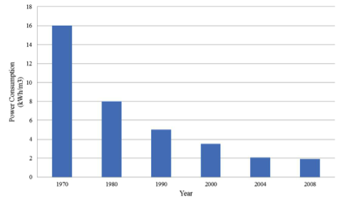
Text description of Figure 3 Image.
| Year | Power Consumption (kWh/m3) |
|---|---|
| 1970 | 16 |
| 1980 | 8 |
| 1990 | 5 |
| 2000 | ~3 |
| 2004 | 2 |
| 2008 | ~2 |
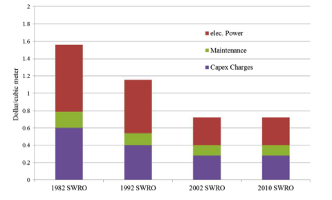
Text description of Figure 4 image.
| Year | Electric | Maintenance | Capex Charges | Total |
|---|---|---|---|---|
| 1982 | 0.7 | 0.2 | 0.6 | 1.5 |
| 1992 | 0.6 | 0.15 | 0.4 | 1.15 |
| 2002 | 0.3 | 0.1 | 0.3 | 0.7 |
| 2010 | 0.35 | 0.1 | 0.3 | 0.75 |
Activate Your Learning
Current water rates (cost for the consumer) in Las Vegas are $1.16 per 1000 gallons. From the data shown in Figure 4, calculate the typical cost of SWRO per 1000 gallons for 2010. Do the same for 1982. How much higher are SWRO costs than current water rates in Las Vegas for the two cases (i.e. are they double the cost? Triple? Ten times?). (Hint: You’ll need to convert between m3 and gallons: one m3 is equivalent to 264 gallons.
1982: $1.55/m3 x 1m3/264 gallons = $0.0059/gallon x 1000 gallons = $5.90/1000gal. This is about 5 times the cost of typical water delivery in Las Vegas.
2010: $0.93/m3 x 1m3/264 gallons = $0.0035/gallon x 1000 gallons = $3.50/1000gal. This is about 3 times the cost of typical water delivery.
Water Re-Use
Water Re-UseAs we’ve already seen in Module 8, one increasingly viable strategy to address limited water supply is that of treatment and re-use. This can take a variety of forms, including reclamation and re-use of wastewater for industrial or consumptive applications like golf courses or parks, or treatment of wastewater to meet drinking water standards and re-use for domestic/municipal supply. The former constitutes a major element of Las Vegas’s approach to maximizing their limited allocation of CO river water from Lake Mead. The latter is becoming increasingly – though not universally - accepted as a way to increase supply, and has been implemented in several areas, including Orange County and even at Penn State!
The Orange County Groundwater Replenishment System (GWRS) is one well-known case study of wastewater reclamation for municipal supply at a relatively large scale (Figures 5-7). The GWRS plant is a 70 million gallons/day facility (72,000 acre-feet/yr) and generates enough potable water for ~500,000 people. The facility also solves the secondary problem of managing effluent to the ocean because much of the wastewater that would otherwise be discharged offshore is captured and re-used. The facility takes advantage of proximity to the wastewater treatment facility to allow for low-cost and efficient “on-site” treatment and uses gravitational energy to transfer the water for treatment. The cost of the facility was subsidized by grants. With the subsidy, the cost of treated water is \$400-500/acre-foot; even without the subsidy, the cost is competitive with imported (CO River) water at \$800/acre-foot.


Two key advantages to reclamation and re-use are: (1) the supply is by definition local, in that it was used by the same people who would use it again, and has already been captured for treatment. This substantially reduces the need for infrastructure and conveyance, and thus is highly efficient and reduces cost; and (2) the total dissolved solids (TDS) in wastewater are much lower than in seawater, such that the energy and cost are low in comparison to SWRO (Figure 8).

Text description of Figure 8 image.
| Type | kWh per million gallons (range) |
|---|---|
| Seawater desalination | 13000-17000 |
| Imported water (state water project/So. Cal) | 8000-15000 |
| Imported water (CO river aqueduct/So. Cal) | 6000 |
| Recycled water (membrane treatment) | 3000-8000 |
| Brackish water desalination | 1000-9000 |
| Imported Water (Northern California) | 0-3000 |
| Recycled water (tertiary treatment) | 1000-2000 |
| Local surface water | 0-1000 |
Another more local example is that of the Penn State “Living Filter”, which has been in operation since the early 1960s, and in full-scale operation since the mid-1980s. The treatment facility captures approximately 2.5 million gallons per day (the total water use on campus at the University, plus a small proportion of water used by residents of the nearby Borough of State College). This water is originally sourced from a fractured limestone aquifer that underlies the region. Rather than treating the wastewater and discharging it to local surface waters (Spring Creek), the water undergoes primary and secondary treatment, followed be de-nitrification and minimal chlorination to ensure that any (unlikely) remaining pathogens in the water are killed, and then spray application in the aquifer recharge area. After treatment, the biological oxygen demand has been reduced by 95-99%. The term “living filter” refers to the thick (>50-75 foot) soil column that overlies the aquifer; the combination of physical processes in the soil, natural degradation by exposure to soil acids and UV, and microbial activity effectively “filter” the treated wastewater to meet drinking water standards. In total, the system is almost 100% efficient in the re-use of extracted groundwater, with ~1 billion gallons of treated water per year recharged to the aquifer.
Of course, there are some obvious drawbacks to water re-use, though these are arguably mostly psychological and rooted in the so-called “Yuck Factor”. It is easy to forget that water is the ultimately reused product. The water in our rivers and oceans has certainly cycled through many organisms over the course of its history (think “dinosaur pee!”). The surface water that we think of as “clean” and which has historically been the dominant water supply for human consumption, hospitals, laundry, and other uses, is mixed with discharged treated wastewater from upstream communities. For that reason, we treat surface water before use. In this sense, why or how is directly treated wastewater any different? Likewise, rural domestic wells are often down-gradient of septic systems or leach fields, albeit a safe distance to allow natural degradation and filtration in the soils and aquifer system. Fundamentally, this raises the question of whether we would rather drink and do our laundry with water that was once our own wastewater, or somebody else’s.
Water Banking and Optioning of Water Rights
Water Banking and Optioning of Water RightsAs we covered in Module 8, one additional hedge against fluctuation in supply, and/or against climate change, is to purchase, trade, or bank water, either using one’s own allocated water in times of surplus or through the purchase of someone else’s unused water rights in a given time period. For example, Las Vegas has adopted this strategy to provide alternate sources in times of severe water shortage, through agreements with Arizona and California. These agreements are one means to transfer water, either actually or virtually, from areas where it is available (in surplus or actively stored in aquifers) to those where it is needed.
More sophisticated arrangements have also been explored, in which water is treated as a commodity and with prices determined by demand. One example of this is described in the High Country News piece "LA Bets on The Farm". The basic concept is that the MWD of Los Angeles pays farmers with water rights for irrigation to fallow some portion of their land. Because, at least currently, there is no shortage of food, the exchange works: LA gains an additional water supply, and the farmers or irrigation districts make a bit of money (without having to take on any risk associated with growing crops, commodity prices, or the like). A more recent iteration of the agreement provides both parties with additional flexibility to account for unpredictable precipitation patterns and water supply, whereby the MWD purchases “options” to the water rights for $10/acre-foot. By March of that particular year, the MWD must decide whether they will take the water or not. If they do, they pay an additional $90/acre-foot (enough that the irrigation districts make some money); if not, there’s still time to plant crops, and the irrigation district keeps the option fee.
At their core, these approaches use the market to define the pricing of water and to shape the terms of agreements that will be mutually beneficial. In part, they work because the amount of water needed for irrigation far exceeds that for municipal or domestic uses (see Module 1). And in part, they work because the irrigation districts receive water that has been heavily subsidized, largely through public investment in major infrastructure that underlies the water systems. Ultimately, however, it is not clear that the exchange or purchase of water rights will really work in the face of severe drought, major climate changes, or continued increases in demand. After all, these strategies are essentially a form of regional water re-allocation or transfer – but in a zero-sum game, they can only work if there is enough surface water or groundwater to be had.
Recognition that these strategies may ameliorate shortages and can serve as a valuable hedge against variability in supply, but are unlikely to fully solve problems of water scarcity if we insist on continued development in water-poor regions, has led to large-scale proposals to transfer water or exchange water rights over great distances and across borders. For example, as discussed briefly in Module 8.1, and in Chapter 3 of The Big Thirst, Las Vegas has begun to explore distant sources of water. These include groundwater in Central and Northern Nevada (a project currently underway), as well as proposed exchanges in which Las Vegas would bankroll desalination facilities in Coastal California, and trade the “new” supply of desalinated water for withdrawal of the same amount from Lake Mead. As described in the next section, the basic fact that there is water available if one reaches far enough – and is willing to pay for it - has led to all manner of proposals to move water across oceans and continents. To an extent, this calls into question Fishman’s assertion that all water problems and their solutions are “local”.
Activate Your Learning
Explain (~100 words) why water banking or optioning is not a viable long-term solution to water scarcity in the case of prolonged water shortage related to sustained severe drought or climate change.
Answer/talking points: Should note that these approaches are no more than water trades, either with other end-users at the current time, or for future water access or rights. These strategies, therefore redistribute or reallocate water to meet the greatest or most severe demand. But if there is simply not enough water to meet demand on a long-term basis, reallocation cannot solve the problem.
Distant Sources
Distant SourcesIf you have ever carried your water on a camping or backpacking trip, you know first hand that water is heavy, and therefore that transport is costly and energy-intensive (that’s why there is a market for water filters and iodine tablets!). For example, almost 20% of electricity in California is used for the water-related activity, and much of that to move water across the state. Despite the high energy and economic cost to transfer large volumes of water, it remains the only – and ultimate – hedge against uncertain supply. As you’ve heard from Marc Reisner and George Miller in the Cadillac Desert films we’ve watched, the idea behind many ambitious water proposed water projects in the Western US, many of which never reached fruition, was to “go where there was so much water, you’d never run out”, and construct “pipelines beyond the wildest imagination”. Patricia Mulroy has even suggested that water transfers from the Great Lakes to the American Southwest should be considered in order to serve the greatest good; water rights and export form the Great Lakes watershed is, not surprisingly, a controversial topic.
In most instances, large-scale water transfers over huge distances by pipeline or tanker are simply too expensive to make sense, or there is too much political resistance. As one extreme example, in the early 1990s, Walter Hickel (then governor of Alaska) and California congressmen Edward Roybal and George Brown requested a feasibility investigation for a pipeline that would bring water from Alaska to California through a subsea pipeline (Figure 9). The committee estimated that the cost of water transfer would be between $3000-4000 per acre-foot, or approximately triple to quadruple the cost of SWRO desalination. In the same report, the committee assessed other sources of water for California and noted that bringing water in by tanker would cost $1,500-2,000 per acre-foot for contracts of at least 30,000 acre-feet.
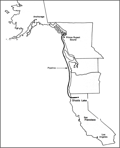
In other cases, the economics are not as prohibitive. For example, water is routinely transferred within California, or between Western States (e.g. Colorado River water transferred to Southern CA in the All American Canal) over distances of hundreds or even over a thousand km. This so-called “imported water” is the basis for the cost comparison of alternative supplies. At a yet larger scale, China has recently undertaken the world’s largest water transfer project, the South-to-North Water Diversion Project (or SNWDP). The main driver for the water project is that precipitation, and thus water resources, are very unevenly distributed across China (Figure 10) – and water-scarce provinces account for over 40% of the GDP. At the same time, almost a third of the population (300 million people) have access only to contaminated water – largely because of insufficient clean water supply and/or limited surface water flows that do not flush pollutants from the channel (as discussed in Module 5 – sidebar on the Three Gorges Dam).
The SNWDP will move almost 45 billion m3 of water per year (36 million acre-feet, or ~3 times the Colorado River’s flow), over distances of almost 4500 km. Although the financial benefits seemingly outweigh the costs – and hence the project is moving forward – major drawbacks are inevitable. For example, such a large water transfer is likely to have major impacts on river systems, in terms of changes in flow, sediment transport, and flushing; relocation of people along the route; construction across archeological and religious sites; and environmental impacts on wetlands that may disappear and endangerment of species that have adapted to the natural river flow regime (sound familiar? think back to Modules 3, 4, and 5!)

.png#mediaviewer/File:China_average_annual_precipitation_(en).png)