Module 4: Sea Level Rise
Module 4: Sea Level RiseIntroduction
You have no doubt seen numerous references to sea level rise, in the media and elsewhere, in recent years. With 60% of the world’s population living within 60 miles of the coast, the current rates of sea level rise – 3.2 mm/yr. (~0.12 inches), and a predicted of sea level rise of approximately 1 meter (39 inches or 3 feet, 3 inches) before the end of the 21st century - we know there will be serious consequences. Such phenomena as king tides, sunny day flooding that occur when there is a new or full moon, accelerated beach erosion, higher and more destructive storm surges, and salt water intrusion into freshwater wetlands and aquifers are a few of the effects that we are hearing about more and more frequently. As these effects persist, difficult questions about the future of some coastal communities will have to be addressed by municipalities, local governments, states, and the federal government, and are indeed already being addressed. In fact, there are many examples around the U.S. and the world of ways in which sea level rise is becoming a persistent problem for residents, and plans and policies to address the issues are being implemented.
In this module, we will examine sea level change at various temporal and spatial scales to gain a perspective and understanding of these current issues. In later modules, we will look at case studies in which sea level rise plays a major role in the daily lives of people in communities around the U.S. and the world and consider the implications for the future of these communities.
Required Video
Begin by watching the following 6-minutes 20-second video Rising Sea Levels - Changing Planet from the National Science Foundation. Learn and make notes on the main takeaway points. These points will recur in this module Note: the narrator incorrectly says that 3 mm of sea level rise is equivalent to 1.2 inches. It is actually 0.12 inches.
Rising Sea Levels
ANNE THOMPSON, reporting:
The shoreline, where the land and the ocean meet; here 60 percent of the world's population live and work within 60 miles of the coast; making rising sea levels a very big threat. For centuries, global sea levels have remained mostly constant. But over the past 100 years, as the climate has warmed, sea level rise has accelerated, rising by about 7 inches, or 17 centimeters. And scientists predict it will only increase. Their models show that over the next 100 years, the seas could rise anywhere from 7 inches to more than 3 feet (18 centimeters to more than a meter) with potentially disastrous social and economic impacts.
Dr. BENJAMIN P. HORTON (University of Pennsylvania): If we get rates of sea level rise greater than one meter, you're going to inundate many of the coastal areas on our planet, causing health problems, socioeconomic problems, biological problems, even political instability.
THOMPSON: Dr. Ben Horton, at the Sea Level Research laboratory at the University of Pennsylvania, says the impacts of rising sea levels are already being felt. Many island nations genuinely worry that their countries are at risk of disappearing altogether. To dramatize the problem, the Maldives government even held a cabinet meeting underwater. In the United States, coastal communities are also worried, with many of its largest cities sitting right at waters edge. Boston, New York City, Washington, DC, Miami, New Orleans, and Los Angeles are only some of the places that face the threat of greater storm surges, flooding, and coastal erosion.
Dr. HORTON: We're trying to look at the globe and say, well, where on our planet shall we be most worried about? Is it the Mississippi Delta? Is it the Nile Delta? Is it going to be Bangladesh with its huge areas of coastal lowlands with high population there? Is it some of the deltas around China?
THOMPSON: Scientists cite two main causes for rising sea levels: a warming climate that is heating the ocean and causing the volume of water to expand, and melting land-based ice sheets and glaciers that are adding to the total amount of water in the oceans.
Dr. DAVID HOLLAND (New York University): Sea level is rising; and of the sea level that we look at today, one third of that comes from warming of the ocean. The other two thirds come from adding water to the ocean.
THOMPSON: Scientists have long known that the warming atmosphere is causing ice sheets and glaciers to melt and flow toward the ocean. But recently, they have discovered that some ice sheets don't just melt from the top.
Dr. David Holland, at New York University's Center for Atmosphere Ocean Science, studies marine ice sheets in Greenland and Antarctica. Marine ice sheets rest on the ocean floor and can melt from both above and below sea level.
Dr. HOLLAND: You can melt ice two ways. You can melt it from the top using the atmosphere or, turns out and more importantly for quick change, you can melt it from the bottom by ocean waters. We have warm waters that are near those ice sheets, and if those warm waters actually touch the marine ice sheets, the marine ice sheets melt, and you have big changes in sea level.
THOMPSON: As the marine ice sheets melt, the land-based ice behind them moves more quickly toward the sea, and this poses the greatest threat for rapid sea level rise. To understand how and why warm ocean water is circulating to Antarctica, Holland devised a rotating water model. He uses ice and cold water for the polar region and warmer water to represent tropical waters, and adds blue and red dyes to represent cold and warm water.
Dr. HOLLAND: What we are really trying to understand is these warm ocean currents, will they actually touch the ice sheets more in the future or less? That-- that's the issue.
THOMPSON: NASA satellites have shown that since 1993, global sea levels are rising at an average of nearly 3 millimeters, or about 1.2 inches, per year. That doesn't sound like much. But when you add in other factors such as local gravity and ocean currents, sea level rise can vary, greatly influenced by the geology of the region.
Dr. HORTON: When we're thinking about sea level rise, we must also consider the land. And the land level changes will differ in relationship to ice age processes, sediment compaction, consolidation, groundwater withdrawal, et cetera.
THOMPSON: Horton and his team take sediment cores from the salt marshes along the U.S. eastern shoreline to study historical sea levels. By analyzing the sediment and microscopic flora and fauna found in the cores, they can determine when sea levels changed dramatically.
Dr. HORTON: And if you look along the core, you've got changes in color that reflect changes in organic content. Each one of these changes marks a change in sea level.
THOMPSON: Horton uses the sediment cores to create a timeline that goes back thousands of years, long before sea levels were recorded by instruments, to gain an idea of how sea levels and land levels have changed.
Dr. HORTON: If we go back through our geological record, the coastline systems have always evolved. As a society, we have to learn to adapt to this dynamic nature of our coastlines. We cannot just say we're going to hold a line.
THOMPSON: Using the past to help people meet the challenges of the future, so we can plan and prepare for the changes in our planet.
Learning Check Point
After watching the video, please take a few minutes to think about what you just learned, and answer the questions below.
As we discussed in Module 1, many coastal cities and smaller communities are increasingly vulnerable to coastal flooding, and sea level rise is a major concern for residents, businesses, and planners. The video mentioned multiple types of issues faced in a future with increasingly higher sea levels, including health problems and political unrest. In this module, we will explore the science behind the causes and effects of sea level change through Earth’s history and examine the recent sea level trends in the context of challenges facing coastal human communities, landscapes, and ecosystems at present.
The following is a NASA video (1:58) showing animation of sea level anomaly data. The data visualization introduced in the video demonstrates that in some areas sea level has risen, while in others it has fallen. Overall, the trend is a global increase in mean sea level, with an increase in the rate of sea level rise.
The current average rate of sea level rise of close to 3 mm per year does not sound like a lot, but it represents an approximate tripling of sea level rise rates since the beginning of the 20th Century. (1900 rate was approximately 1.4 mm/ year on average, now it is more than 3.4 mm/ year on average).
Video: 22 Years of Sea Level Rise Measured From Space(1:58)
This visualization shows total sea level change between 1992 and 2014, based on data collected from the TOPEX/Poseidon, Jason-1 and Jason-2 satellites. Blue regions are where sea level has gone down, and orange/red regions are where sea level has gone up. Since 1992, seas around the world have risen an average of nearly 3 inches.
Hi! I'm Josh Willis, the project scientist for the Jason-3 missions to measure sea level rise from space.
In some ways, sea level rise is really simple. As water heats up, it takes up more room. This drives sea level rise and, in addition, as glaciers and ice sheets are melted, extra water is added to the ocean, just like when you turn on your faucet in the bathtub.
Over 90 percent of the heat trapped by greenhouse gases is being absorbed by the oceans. When that happens, seawater expands, and this helps drive sea level rise.
Hundreds of millions of people around the world live on coastlines that can be threatened by rising seas. This animation shows how sea levels have changed over the last 23 years. Globally, sea levels have gone up by about 6 centimeters during that time, but it doesn't happen all at the same speed everywhere. Some places are rising faster than others, and some places are even falling.
Orange and red colors mean that sea levels have gone up in these locations, and blue and white means sea levels stayed the same or actually fallen. We can see that most places in the ocean are orange, meaning sea levels risen over the last 23 years. In a few places, you can see blue where sea level has actually dropped. Here, we see the Gulf Stream. The red and blue indicate that this massive current has shifted slightly in the last 23 years off the west coast of the United States. We've seen sea levels actually drop. This is because waters there have been cooling because of something called the Pacific decadal oscillation. In the western Pacific, sea levels have been rising very rapidly. This is because of heat being pushed from east to west across the Pacific. Sea level rise is going to be a major impact of human-caused climate change and, here at NASA, we're doing everything we can to try and better understand it.
Credit: VideoFromSpace
Goals and Objectives
Goals and Objectives- Students will develop fundamental geospatial skills and concepts needed to assess coastal processes that produce sea level change.
- Students will be able to explain what sea level is and differentiate the mechanisms that interact to produce changes in sea level over short-term and long-term time periods.
- Students will characterize trends in sea level over geologic time and conceptualize how changes in sea level can result in various spatial scales of coastline change.
- Students will use real tidal gauge data from diverse regions to identify recent trends in sea level change, and will use these trends and NOAA Sea Level Rise Viewer data to formulate projections for future sea level positions.
Learning Objectives
By the end of this module, students should be able to:
- describe the changes in sea level change in the Earth’s geological history, to gain a perspective of modern sea level rise;
- distinguish among methods used to determine sea level changes taking place in the past, present, and future;
- identify factors (intrinsic, extrinsic, and anthropogenic) that contribute to sea level change;
- discriminate among causes of local, regional, and global sea level change and associated impacts on coastal morphology and human communities;
- locate and use key datasets and data visualizing tools to analyze sea level dynamics at different temporal scales, and their impact on coastal landforms.
Module 4 Roadmap
| Activity Type | Assignment |
|---|---|
| To Read | In addition to reading all of the required materials here on the course website, before you begin working through this module, please read the following required readings to make sure you are familiar with the content so you can complete the assignments.
Extra readings are clearly noted throughout the module and can be pursued as your time and interest allow. |
| To Do |
|
Questions?
If you have any questions, please use the Canvas email tool to contact the instructor.
What is Sea Level and How is it Measured? An Introduction
What is Sea Level and How is it Measured? An IntroductionThe following pages look at what sea level change is, and what mechanisms drive sea level change on a planetary scale.
Before we investigate these mechanisms further, let’s ask a couple of fundamental questions: What is sea level anyway? How is it measured...and why has it fluctuated during the course of geologic time? And why is it not even across the globe? As you watch the following quick video, make a list of forces mentioned that influence sea level. The video clip (3:25) was published on Nov. 25, 2013, by MinutePhysics.
Video: What is Sea Level? (3:25)
What is Sea Level?
Sea level seems like a pretty easy concept, right? You just measure the average level of the oceans and that's that. But what about parts of the Earth where there aren't oceans? For example, when we say that Mt. Everest is 8850m above sea level, how do we know what sea level would be beneath Mt. Everest, since there's no sea for hundreds of kilometers? If the Earth were flat, then things would be easy - we'd just draw a straight line through the average height of the oceans and be done with it. But the Earth isn't flat.
If the Earth were spherical, it would be easy, too, because we could just measure the average distance from the center of the Earth to the surface of the ocean. But the Earth isn't spherical - it's spinning, so bits closer to the equator are "thrown out" by centrifugal effects, and the poles get squashed in a bit.
In fact, the Earth is so non-spherical that it's 42km farther across at the equator than from pole to pole. That means if you thought Earth were a sphere and defined sea level by standing on the sea ice at the North Pole, then the surface of the ocean at the equator would be 21km above sea level. This bulging is also why the Chimborazo volcano in Ecuador, and not Mount Everest, is the peak that's actually farthest from the center of the Earth.
So, how do we know what sea level is? Well, water is held on Earth by gravity, so we could model the Earth as a flattened & stretched spinning sphere and then calculate what height the oceans would settle to when pulled by gravity onto the surface of that ellipsoid. Except, the interior of the Earth doesn't have the same density everywhere, which means gravity is slightly stronger or weaker at different points around the globe, and the oceans tend to "puddle" nearer to the dense spots. These aren't small changes, either - the level of the sea can vary by up to 100m from a uniform ellipsoid depending on the density of the Earth beneath it.
And on top of that, literally, there are those pesky things called continents moving around on the Earth's surface. These dense lumps of rock bump out from the ellipsoid and their mass gravitationally attracts oceans, while valleys in the ocean floor have less mass and the oceans flow away, shallower.
And this is the real conundrum, because the very presence of a mountain (& continent on which it sits) changes the level of the sea: the gravitational attraction of land pulls more water nearby, raising the sea around it. So, to determine the height of a mountain above sea level, should we use the height the sea would be if the mountain weren't there at all? Or the height the sea would be if the mountain weren't there but its gravity were?
The people who worry about such things, called geodetic scientists or geodesists, decided that we should indeed define sea level using the strength of gravity, so they went about creating an incredibly detailed model of the Earth's gravitational field, called, creatively, the Earth Gravitational Model. It's incorporated into modern GPS receivers so they won't tell you you're 100m below sea level when you're in fact sitting on the beach in Sri Lanka which has weak gravity, and the model has allowed geodesists themselves to correctly predict the average level of the ocean to within a meter everywhere on Earth. Which is why we also use it to define what sea level would be underneath mountains... if they weren't there... but their gravity were.
The Minute Physics video introduces a few key concepts that make measuring sea level pretty complex:
- The Earth is not perfectly spherical, but an ellipsoid, due to its spin. This means that the Earth is “fatter” at the equator and slightly flattened at the poles, so that: “if you thought Earth was a sphere and defined sea level by standing on the sea ice at the North Pole, then the surface of the ocean at the equator would be 21km above sea level”.
- Differential density of the interior of the Earth so that “gravity is slightly stronger or weaker at different points around the globe, and the oceans tend to "puddle" nearer to the dense spots”.
- The mass of the continental plates creates a greater gravitational pull on ocean water than the ocean basin so that “mass gravitationally attracts oceans, while valleys in the ocean floor have less mass and the oceans flow away, shallower”.
These phenomena mean that there are peaks and valleys in the surface of the ocean – the ocean level is not uniform across the planet. These are important concepts to keep in mind as you read on.
We will also meet several other phenomena that drive sea level changes around the planet later in the module.
Sea Level Definitions
Sea Level DefinitionsIn a perfect, non-moving, homogeneous sphere, the elevation of the Earth's liquid shell would be distributed equally about the center of gravity, and sea levels would be the same everywhere. However, the Earth is a heterogeneous, oblate spheroid that rotates on an axis and experiences gravitational influences from other planets and the sun. These factors, together with geographic variations of continents and submerged terrains, climate systems, water volume, tectonics, etc., the surface of the ocean, and hence sea level, change on various time scales, ranging from minutes to millennia. Therefore, it is a challenge to determine the exact sea level of the Earth, but it is done.
As a result of these complications when referring to sea level, geoscientists have to be a little bit more specific when they discuss "sea level." Hence, there are a number of different definitions for "sea level" that need to be understood.
- Global Sea Level - the average height of the Earth's oceans combined (relative to the Earth's center). Influenced primarily by the factors that influence the volume of seawater, and size of ocean basins, etc. Often referred to as "Eustatic Sea Level"
- Local (or regional) Sea Level - the height of seawater relative to a fixed point on land that is used as a continuous reference. Influenced by meteorological factors, tidal range, ocean currents, rates of subsidence/uplift. Also referred to a "Relative Sea Level"
- Mean Sea Level (MSL) - the average height of seawater relative to a fixed datum established by a statistical average of water heights over a period of time. This is the most functional definition for sea level because it helps establish the elevation of all points on Earth (topographic elevation, and bathymetric elevation). In the U.S., MSL is often reported relative to the 1983-2001 NTDE (National Tidal Datum Epoch). Tidal datums need to be updated every couple of decades because sea level is not stable, and a new datum is likely to be announced.
Measuring Sea Level
Measuring Sea LevelMeasuring Sea Level Using Tide Gauges
Measuring sea level using gauges has a 200-year history. Today, the technology has changed, but the principles are the same as before, and some gauges provide very long and reliable records of water levels that can be used to observe sea level change trends. For example, the Fort Point tide gauge in San Francisco has more than 100 years of record that we will access later.
Sea level is often measured locally by tide gauges (and averaged over tidal cycles) that detect high and low points in a given period of time. Local tide gauges are especially useful for people who work or recreate in coastal areas and need to know what the water level ranges will be. These data points are also important for detecting water levels during storms and other events, as well as in the long-term investigation of relative water level change (rise or fall). Tide levels are also measured by floating buoys, which may also be used to detect tsunami waves. We will use tide gauge data to investigate sea level changes in different locations in the Module 4 Lab.
Measuring Sea Level Using Satellite Altimetry
With the advent of satellite altimetry in the 1960s, measurements of the sea surface took on a whole new level of accuracy. Between 1996 and 2006, altimetry took off with multiple satellites orbiting the Earth, providing much better coverage and data resolution. These measurements utilize multibeam methods that are very precise and can measure changes in elevation on the Earth's surface to great precision in the range of centimeters. These methods have shown that water bodies are not flat, but are incredibly dynamic and have high and low spots due to factors such as gravitational variability described above. Data such as ocean circulation, sea level rise, and wave heights can be measured. These measurements have provided insight into the links between the ocean and the atmosphere and how the connections drive climate. Satellite altimetry data collection began in earnest with the launch in 1992 of the TOPEX/Poseidon joint satellite mission between NASA and CNES, the French space agency. TOPEX/Poseidon proved data previously impossible to obtain. The next generation of satellites to collect these data was the NASA Jason satellites. They have been collecting data since Jason 1 was launched in 2001. Jason 2 was launched in 2008, while Jason 3 is presently collecting altimetry data. Each mission lasts about 5 years. Meanwhile, the European Space Agency’s Sentinel 3 satellite is collecting similar data, as shown below.

How Satellite Altimetry Works
As the figure illustrates, satellite altimetry measurements are obtained by a system of instruments carried on a satellite orbiting the Earth. The instruments include an altimeter and antenna, which measure sea surface height; a radiometer, which measures atmospheric disturbances, and a GPS system for precisely determining the satellite’s location. The altimeter transmits rapid (1700/second) pulses of microwave energy towards the Earth, which reflect back to the satellite. The average round-trip time of these pulses is accurately measured to determine the exact distance between the satellite and the sea surface (range). Water vapor measurements are also made as the level of water vapor affects the rate of transmission of the pulses, and a correction must be made to obtain the final range, which is accurate to 2 cm. This range must be referenced to the reference ellipsoid, which is an approximation of the Earth’s surface (the sphere flattened at the poles discussed above). The GPS receiver onboard and ground-based radio receivers track the satellite’s exact location. Using these data, sea surface height can be accurately measured. In addition, the ocean surface topography (the highs and lows depicted on the images) are obtained through calculations. This information is key to understanding the ocean’s surface as a dynamic and complex terrain and to determining changes over time.
The Jason satellites have revealed critically important information that was not available prior to the mid-1990s. As technology develops and more data are added to the database, our understanding of the changing ocean increases. Among the many scientific goals of the Jason and other altimetry satellite systems currently in use, are to extend the time series of ocean topography measurements begun in 1992 and to monitor the changes in global mean sea level and its relationship to global climate change. Since the mid-1990s, there has been explosive growth in ocean and climate studies, and multiple altimetry satellites have provided longer and more accurate measurements and have led to better spatial and temporal coverage and resolution. These accurate and detailed measurements, in turn, inform predictive science on sea level change.
In addition, important information on ocean circulation and the relationships between heat transport and other variables such as nutrients and salt content are obtained, as well as measurements of wave height. These data can be used in modeling that informs our understanding of tides, weather, and other dynamic phenomena at work on our planet. This technology continues to add knowledge and understanding of our ocean.
Recommended Reading
More detail on the Jason mission can be found at Jason-3 NASA Sea Level Change Portal.
The uneven nature of the surface of the ocean is expressed in the maps below. These images were compiled from satellite altimetry data to show anomalies in sea levels and temperature. These types of data are used in sea level predictions. The complex science involved in tracking sea levels is evolving rapidly as it answers a pressing need to provide accurate predictions in a rapidly changing world.

Sea Level Change: What are Anomalies and Why are They Used in Climate Change Analysis?
Sea Level Change: What are Anomalies and Why are They Used in Climate Change Analysis?If you are interested in understanding climate change, and you pay attention to in-depth news stories on the topic, you have no doubt frequently heard or read references to sea level and temperature anomalies. Anomaly data are being shared with greater regularity in the media these days, so it is important to understand what we mean by terms like sea surface temperature anomalies and sea surface height anomalies. An anomaly is an inconsistency or deviation from the norm, so images are created to show where change is taking place in the ocean in either a positive or negative trend when comparing to previous data. This is sometimes referred to as Sea Surface Height Deviation data or SSHD. Sea surface height anomalies are calculated using data from satellite altimeters. Many years’ worth of thousands of measurements provide a historical mean sea surface height, and the difference between the historical mean and the sea surface measurement for a particular date is called the sea surface height deviation. This can be calculated for points over the ocean surface, providing the data for the incredible maps we are seeing that show color-coded variations in sea surface across the globe and the changes in these measurements over time and space.
In the figure below, the data show the sea surface height differences compared to the 1961 – 1990 average over the entire planet. By comparing sea surface height measurements for a particular time period with the average measured over a previous time period, the changes can be shown spatially. In the figure below, the warm colors are sea surface heights that are significantly greater than past measurements, while the cool colors are those areas showing significantly lower elevation in the sea surface. This is how sea level rise trends can be identified in different parts of the globe using satellite data.
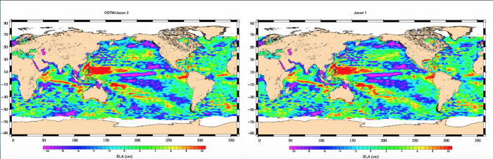
Revisit the NASA animation "22 Years of Sea Level Rise Measured from Space" from the Module 4 Overview that shows a 22-year period of sea level change using anomaly data. It is an excellent quick visualization of these phenomena.
Putting Sea Level Change in Context of the Earth’s History
Putting Sea Level Change in Context of the Earth’s HistoryThinking in the Long Term: Sea Level Change in Geologic Time
The instrumental data we explored above gives a small window of time in Earth’s recent history. To put the recent changes into context, we need to also consider long term changes in sea level.
Humans typically have difficulty thinking about time beyond a human lifespan. Geologists may be the exception to this rule, but you may belong in the category of those who find it difficult to visualize the long distant past and the long distant future and to think in terms of millions or billions of years (or even thousands of years). But understanding the changes to atmospheric and ocean changes in the geologic history of the Earth is important if we are to understand what is going on with our climate and sea levels today.
Thinking REALLY long term: Below is a graph plotting sea level over the past 540 million years - since the Cambrian era. For reference, zero on the Y-axis is where the current sea level is. We don’t need to go into a lot of detail, but you can easily appreciate that sea levels have been much higher than today for much of this period of the Earth's history. Scientists have correlated these fluctuations with changes in atmospheric carbon dioxide and ocean and atmospheric temperatures, using methods described in the next few pages.

We also must acknowledge here that some people may argue that sea levels have always fluctuated, so why is sea level rise today a big deal? Hopefully, we can shed some light on this question by looking at the changes in sea level through the history of the Earth, while considering the causes for these changes. But, perhaps the simple fact that seas are rising faster than ever before in human history is enough to facilitate action and adaptation. You also may ask, “What can we do about it?” This question will be addressed in later modules.
For a rapid and fun overview of the history of the Earth’s climate changes, watch the following fascinating monolog video. It summarizes most of the concepts to be discussed in more detail in the materials that follow.
Video: A History of Earth's Climate (11:19)
A History of Earth's Climate
We sometimes forget that this planet had a climate long before we showed up and started noticing it and then eventually affecting it, but let's be clear. The climate of this planet has always been pretty not so -- ice ages, completely iceless ages, volcanic winters, crazy methane, and ammonia atmospheres -- you name it. Our climate is influenced by a whole series of cycles, some incredibly long, some lasting only a few thousand years. These cycles have been churning along for hundreds of millions of years, and in most cases, they'll continue long after we are gone.
A look at the history of climate change on Earth can give us some much-needed perspective on our current climate dilemma because the surprising truth is what we're experiencing now is different than anything this planet has encountered before. So, let's take a stroll down Earth's climate history lane and see if we can find some answers to a question that's been bugging me a lot lately -- just how much hot water are we in, exactly?
Over the past 540 million years or so, Earth's environment has experienced a few large fluctuations between two very different states: greenhouse and icehouse climates. During greenhouse periods, there's a lot more liquid water on the planet and very little, if any, ice at the poles. During icehouse conditions, the global climate is cold enough to support large sheets of ice at both the poles. The most recent transition between these phases occurred about 55 million years ago when Earth reached thermal maximum, the peak of its last greenhouse state. Back then, there were turtles and palm trees at the poles, and the equator, we can assume, was pretty inhospitable. Then a long process of cooling started, ultimately resulting in an ice age that we are currently experiencing at this very moment. But, of course, Earth's climate doesn't just change for no reason, so what happened?
Well, one theory is that the Arctic Ocean was subject to a huge bloom of freshwater fern called Izola, which eventually died and sank to the seafloor, taking with it a massive load of carbon, which is, of course, coming from carbon dioxide, a greenhouse gas. So, with less carbon dioxide in the atmosphere, the earth began to cool until we landed in a great big ice house. That fern is a good example of how living things can influence the climate over long periods because, over time, there's been a big give-and-take between oxygen, which is manufactured by plants and consumed by animals, and carbon dioxide, which is spewed out by animals and used by plants. The relative abundance of these gases has a lot to do with what the climate is like at any given time. When there's a lot of greenhouse gases like carbon dioxide and methane in the atmosphere, they trap heat to create a greenhouse effect; when there's less CO2 and other greenhouse gases in the atmosphere, the planet cools down. But, of course, when it comes to the really long-term cycles, we have to talk about that all-important climate influencer which you could probably guess at: the Sun, which can affect climate in a bunch of ways.
For starters, the Sun hasn't always been as bright as it is now. When the earth was young, the Sun itself was just a baby -- less than a billion years old and about 70% dimmer than it is today. Nowadays, the Sun has some serious stability, but it still varies a bit. Fluctuations in the sun's energy export run in 11-year sunspot cycles. During periods of maximum solar activity, the Sun emits about 0.1% more energy than during Sun SPOT minimums, so not a lot. The sunspot cycle has at best a subtle impact on earth temperatures. But, on top of that, variations in the Earth's orbit and inclination toward the Sun also cause temperature fluctuations. Over millions of years, the shape of the Earth's orbit around the Sun varies from nearly circular to elliptical. This causes the distance from the earth to the Sun to vary during its orbit and with it the amount of solar energy we receive. This phenomenon is called orbital eccentricity, and it occurs in cycles of about a hundred thousand years. Right now, scientists think we're probably somewhere near the minimum of this cycle with the distance from the Sun only changing slightly in a single orbit enough to create about a six percent difference in solar radiation throughout our orbit. But, when the earth is at the peak of this cycle, the amount of the sun's energy we receive can change as much as 30 percent in a year, which means crazy big fluctuations in climate. While orbit changes, so does the tilt of the Earth's axis as it spins through space. The earth wobbles a bit changing its angle with respect to the Sun and cycles that run about 42,000 years. So, right at this moment, the earth tilts at a twenty-three point four-degree angle, but, over the eons, that can change from as small as 22 point one degree to as much as 24 point five degrees. The steeper the angle, the more the poles are directed toward the Sun, which makes for far greater extremes as the seasons change, with the poles being way warmer in the summer and much, much colder in the winter.
A lot of the changes in prehistoric climate seem to coincide with these cycles, particularly the changes in Earth's orbit, and while nothing is completely certain at this point, many experts think that these orbital cycles have had huge influences on the cycles of climate change that we find in the record of recent geologic history. So, while these are the most general climate influencers that we know about today, it wasn't like this at first. Between 4.5 and 3.8 billion years ago, when the earth was just a baby, there was no climate to speak of. The surface was just molten lava, and it was real hot up in here. After the atmosphere eventually cooled enough for it to rain, oceans formed and land masses appeared. At that point the Sun was way cooler, but the Earth's atmosphere, which consisted mostly of ammonia and the greenhouse gas methane, kept the planet nice and toasty. Between 2.5 billion and 500 million years ago, oxygen levels rose dramatically. much of the life that had managed to take hold by then was anaerobic or lived without oxygen, but thanks to the evolution and hard work of kajillions of photosynthetic algae called cyanobacteria, which started pumping out oxygen like nobody's business, the composition of the atmosphere changed to the point where a whole lot of anaerobic life couldn't deal. This oxygen boom resulted in the great oxygen catastrophe, one of the most significant extinction events in Earth's history. Well, it was a catastrophe for the anaerobic bacteria in the archaea, but a nice bit of luck for us, who wouldn't happen along for another couple billion years or so. I guess it's all about perspective.
There was probably a big cooling around this time too, partly because of the rise in oxygen and most of the methane being removed from the atmosphere at the peak of this cooling period. It's thought that the average temperatures at the equator were about what they are in modern-day Antarctica. Some scientists think that the entire globe essentially froze, resulting in what they call a snowball earth. Between 500 and 250 million years ago, the planet's core cooled down to the temperature it is today, so volcanic eruptions became rare. It's during this time that we see the Cambrian explosion, where multicellular life evolved like crazy in the oceans. Photosynthetic organisms on land turned out oxygen, but there weren't yet enough aerobic organisms to breathe it in and pump the CO2 back out, so earth stayed pretty chilly.
250 to 65 million years ago, all that changed. By then, there were lots of critters on land exhaling all that CO2. Pangaea, the huge honkin supercontinent, was also starting to break up, so more land was coming into contact with the oceans' increasing humidity and helping drive the climate into a warming period. This culminated at a time when temperatures were about 10 degrees Celsius higher than they are today and pretty uniform all over the globe. Then another climate change driver intervened.
The reigning theory is that 65 million years ago, a 200 kilometer-wide asteroid smashed into what is now Mexico; sprang up nine hundred quadrillion kilograms of flaming rock into the atmosphere. This probably caused an impact winter that was likely enough to kill off all the large dinosaurs and allow mammals to kind of take over. Just ten million years later, we began the run-up to that thermal maximum I mentioned earlier. About 55 million years ago, the planet experienced sudden warming, which sent global temperatures up five to eight degrees Celsius in just 20,000 years. It didn't last very long, and what exactly caused it is a matter of debate, but the geological record shows that there was a huge infusion of carbon into the environment.
One of the most popular hypotheses is that it came from methane being released from sudden melting of methane containing ice under the seafloor and at the poles something happened, say undersea volcanic activity or a peak and one of the solar cycles we talked about, to melt this methane ice. And once it was unleashed into the atmosphere, we were all in greenhouse city. Because of this little escapade, the earth went completely ice-free. The opposite of snowball earth, sometimes called greenhouse earth or hothouse earth, and in addition to creating an ideal climate for warm-blooded creatures like us mammals, this also allowed for the proliferation of more plant life, including that huge bloom of Izola freshwater fern, so levels of greenhouse gases started to tank yet again.
But when the next cooling trend began, this time it was different. About 35 million years ago, glaciers started to form in Antarctica for the first time, in part because there was no Antarctica before. See, while all the cycles that we've been talking about kept churning, the continents were also sliding around on the Earth's surface until land masses appeared at the South Pole that allowed glaciation to take place. Meanwhile, other formations that didn't exist before, like the Himalayas and the Atlantic Ocean, had taken shape, which helped to amplify and circulate the cooling and thus began a major Ice House climate. When people talk about the ice age, this is usually what they mean, and because there's still permanent ice to be found, we're technically still in it.
But this cooling hasn't been consistent within this ice age. There have been small warming events interspersed with even cooler events, where average temperatures were about five degrees Celsius cooler than today. In fact, in the past 2.5 million years there have probably been around 25 glaciations or cold periods, sometimes called little ice ages, interspersed with interglacials which are warmer periods. You might notice that that comes out to about one climate swing every 100,000 years, which coincides with that orbital pattern we talked about and that brings us up to now, or, you know, within about 12,000 years of now, which is yesterday in geologic time.
So, you've heard of the hockey stick, right? This is the graph depicting the average global temperatures over the last two thousand years or so based on what can be gathered from historical data -- tree rings, corals and ice cores -- you'll notice that average temperatures increased dramatically during the 20th century, which is when we started relying heavily on fossil fuels to power our everything. This graph came out in 1999 using data collected by Penn State climate scientist Michael Mann, who has taken an incredible amount of heat for this research over the past 15 years.
But new research reconstructs global temperatures further back than Mann did -- eleven thousand three hundred years back, using fossilized plankton dug up by oceanographers from 70 sites worldwide. On one hand, it shows that temperatures for about 20 percent of this historical period were actually higher than they are today, but it also shows that right now temperatures are increasing faster than they ever have. In the past 100 years, temperatures have risen so dramatically that they have canceled out all of the cooling that took place over the past 6,000 years. And probably more important, the study shows that in addition to being in the middle of a long-term ice age, we should now be entering the bottom of a several-thousand-year-long cooling period even if it were just natural factors, but it's not.
So, this new evidence pretty much corroborates what's already known. That we're making a mess. But one thing's for sure, our planet's climate has dealt with a lot and it'll probably survive humans. But what the cost will be for us? We're going to need some more data on that.
Thanks for watching this episode of SciShow. If you have any questions, comments, or suggestions for us, you can find us on Facebook and Twitter or down in the comments, and if you want to keep getting smarter with us here at SciShow, you can go to youtube.com/scishow and subscribe.
Measuring Sea Level Changes in Earth’s Past
Measuring Sea Level Changes in Earth’s PastSea levels change over different spatial and temporal scales. The images produced by altimetry illustrate well the spatial variations, and also provide important data on relatively recent temporal changes. We can examine sea level changes over the short term and long term. Examination of tide gauge data gives us a detailed look at sea level change over a short period of history. These are valuable, but do not show us the whole picture.
If we want to look back at the planet’s ocean levels before people began making measurements, we must use proxy, or indirect measurement. This is the basis of the science of paleoclimatology. Before looking at more information on paleoclimate, we need to understand how these data are obtained.
Paleoclimatology
How do we know what the climate was like 500 million years ago? To reconstruct and understand the fluctuations in climate that have taken place on Earth, scientists use proxy, or indirect data, including data obtained in ice cores, coral, tree rings, and ocean and lake sediment cores.
Paleoclimatologists use various forms of environmental evidence to understand the Earth’s past climate. Earth’s past climate conditions are preserved in tree rings, skeletons of tropical coral reefs, sediment layers in lakes and the ocean, and in the ice of glaciers and ice caps. Using these records, paleoclimatologists can reconstruct climate conditions going back hundreds of millions of years to create graphs such as the one in Figure 4.4 on the previous page.
It was the examination and analysis of ice cores and their trapped molecular contents that revealed the connection between Earth’s atmospheric CO2 and temperature. In order to unlock the information contained in the ice, scientists collect cores and analyze them in slices representing small increments of time, using very precise methods. This way patterns that identify changes in the atmosphere's composition and temperature can be revealed.
For example, the ratio of oxygen isotopes present in the cores ("light" oxygen-16 to "heavy" oxygen-18) can tell the story of global temperatures when the ice formed. Colder temperatures are needed to produce precipitation when water vapor in the atmosphere contains higher levels of oxygen 16.
The paleorecord shows that the Earth’s climate is always changing and that in the distant past (such as the Cretaceous – think end of the dinosaurs’ reign - from 145.5 to 65.5 million years ago), the climate on Earth was much warmer than today and sea levels would have been significantly higher. See Figure 4.4 on the previous page.
The paleoclimate record also shows that in relatively recent geologic time (within the last 2 million years), the Earth underwent a series of glacial periods, which locked much of the Earth’s water in ice which covered the Northern Hemisphere landmasses. This caused the sea level to drop much lower than today (more than 400 ft. below current levels). We are currently in an “interglacial” period during which the Earth has warmed, and the sea level has risen.
Paleoclimate records can also help to shed light on the more recent changes and provide evidence for the anthropomorphic effects on climate and sea level, correlating an unprecedented rapid rise in sea level with increased carbon dioxide in the atmosphere. More on that later.
Required Reading
Please read the article on how scientists use ice cores to reconstruct past climates, "Climate at the core: how scientists study ice cores to reveal Earth’s climate history".
Sea Level in the Past 200,000 Years
Sea Level in the Past 200,000 YearsLet’s look at how sea levels have changed over the past 200,000 years of Earth’s history, based on evidence provided by paleoclimatology.
Probably, the factor that influences sea levels on the planet more than any other is the proportion of the Earth’s water that is in the form of ice at any point in time.
The figure below illustrates this very well. Take a look at the curve on the graph, obtained by analyzing oxygen isotopes in ice cores. It represents the fluctuations in sea level from 200,000 years ago to the present (going from right to left on the x-axis). Approximately 125,000 years ago, the sea level was approximately 8 meters higher than it is today. This was during the Sangamonian Interglacial, the last time the north polar ice cap completely melted. After this peak in sea level, ice returned to the planet. And the Wisconsinan Glacial period followed between 80,000 and 20,000 years ago when a glacial maximum, and sea level low stand (more than 130 m lower than today) took place. This is what most people mean when they refer to the "ice age". Glaciers covered much of North America. Following the glacial maximum, we see sea levels rising rapidly - the curve is about as steep as the one leading up to the Sangamonian Interglacial. It began to level off about 5,000 years ago, leading to fairly slow sea level rise in recent geologic time and the sea level human society has been accustomed to.


The figure above (Hearty) illustrates the CO2 fluctuations over 400,000 years and the rapid rise to the recently reached 400 ppm level (Keeling curve). These levels are unprecedented during the past 800,000 years. During the Sangamonian interglacial period mentioned above, at about 130,000 years ago, levels reached 300 ppm, but sea level was much higher than today. A CO2 level of 400 ppm occurred in the Pliocene 3 million years ago, when sea level is estimated to have been 10 to 40 m higher than it is now. The concern is that, based on evidence provided by paleoclimate studies such as those illustrated in the two figures above, this rapid increase in CO2 levels can be correlated with the melting of ice sheets leading to an ice-free planet. This melting is currently being watched closely. If all of Greenland’s ice were to melt, an increase of 5-7 m in sea level would be experienced. This is predicted to lead (as well as flooding of all coastal cities on the globe) to the disruption of the circulation of ocean currents (due to the rapid addition of huge volumes of freshwater to the ocean) that currently dictate the climate patterns as we know them in Earth. Of course, the implications of this scenario are huge. Stay tuned, and pay attention when you hear of news related to this phenomenon.
We will return to the ideas presented in these graphs after considering the complex cause and effect mechanisms that control sea levels on the planet.
Learning Check Point
Learning Check PointThere are several takeaways from studying the two graphs on the previous page. Look closely at the data presented and answer the questions below.
Learning Check Point
Causes of Sea Level Fluctuations Through Time
Causes of Sea Level Fluctuations Through TimeWhat were the causes of the changes in sea levels on the Earth over time? There are multiple causes that can be divided into two groups: intrinsic, or internal drivers, originating within the Earth’s system, and extrinsic drivers, which originate outside the Earth’s system. Some of these operate over the timeframe of the Earth’s history, and others operate over shorter timeframes. Some influences are global in scale, while others are more regional or localized. The following pages are part of a partial list of these influences. These drivers are also interconnected, with one influencing another in many cases.
Intrinsic Causes of Sea Level Change
Intrinsic Causes of Sea Level ChangeThe Earth is a dynamic, self-regulating system, and forever changing. The changes that take place in each of the spheres of the Earth impact the other, connected spheres. There are complex feedback mechanisms that work to maintain the balanced functions of the planet. As we explore the topic of sea level change, the importance of these feedback mechanisms become clear. It is hard to isolate a single cause of sea level rise or fall, as all are connected and may be occurring simultaneously. It is worth remembering some principles you may have learned in your pre-college days, such as the water cycle, rock cycle, plate tectonics, and how heating and cooling affect matter.
Global or eustatic sea level can oscillate due to changes in the volume of water present within the ocean basins relative to storage of that water on land. Short-term sea level change can be driven by sudden tectonic events (e.g., earthquake-induced subsidence/uplift), and tidal processes, but sea level change on the scale of decades to 1000s of years is primarily driven by changes in the Earth's climate system that can be influenced by both intrinsic and extrinsic phenomena.
The Water Cycle
The Water CycleAs you probably know, the water on the planet is constantly being cycled through various states, such as water vapor in the atmosphere, liquid water in oceans, rivers, and groundwater, and ice in ice sheets and glaciers. This cycling happens at different rates, from rapidly (measured in days) to very slowly (measured in thousands of years or more).
Whether due to climate factors, or plate tectonic factors, water evaporated from the oceans can become locked up on land and prevented from cycling back to the ocean. The USGS estimates that some 8,500,000 cubic miles of water is trapped on land either as ice or as freshwater. When and if this water makes its way back to the ocean (and if it is not replaced on land), sea levels can rise significantly. The Greenland Ice sheet, if melted, is estimated by Byrd Polar Research Center and other scientists to produce a rise of between 6 and 7.4 meters to global sea level if it is not restored on land.
Rift lakes or large intra-continental seaways can trap liquid water that is temporarily removed from the global ocean (an excellent example is Lake Bonneville - the ancestral Great Salt Lake of the western U.S.). If precipitation of ocean-derived water is high on land, and this water is not able to return to the ocean, ocean water levels can drop over time.

Continental aquifers will often hold volumes of water in the subsurface. As these aquifers are de-watered (pumped), the water is released back into the hydrologic system and can be returned to the ocean. Some areas in large desert regions (e.g., in Arizona, Nevada, California, etc.) have withdrawn substantial amounts of water from aquifers. This water is not replaced, ground subsidence occurs, and the aquifer becomes compacted. The withdrawn water is eventually lost to evaporation and ends up back in the ocean.
Glaciers also trap and hold water in solid form. When ocean-derived moisture freezes and is held on land from year to year, they stockpile large volumes of water, and ocean levels can drop.

Two main types of glaciers include alpine and continental glaciers.
- Continental glaciers or ice sheets similar to those on Greenland, Iceland, or Antarctica have been more widespread at times in Earth's history and trapped large volumes of water on land, so much so that continental areas subsided under the great thicknesses of ice built on top of them.
- Large numbers of alpine glaciers at high altitudes (e.g., Andes, Alps, Himalaya, Cascades, Rockies, etc.) collectively contain significant volumes of water that can also be released back to the global ocean if melted.
Isostatic Changes – Glacial Isostatic Adjustment
Isostatic Changes – Glacial Isostatic AdjustmentTo understand isostatic changes, you need to consider the fact that huge amounts of water can be stored as ice during colder periods in Earth’s history (many times more than today). When the planet warms and ice melts, this water is returned to the ocean basins (causing a rise in sea level). When ice sheets and glaciers covered the land during the ice ages of the Pleistocene, the weight of the ice depressed the elevation of the land. Over the 20,000 years since the last glacial maximum, the land masses, relieved of their burden of ice, have gradually rebounded. This rebound is called Glacial Isostatic Adjustment or GIA. The level of the land relative to the sea level increases. This can cause a regional sea level change effect and is still impacting parts of Alaska and other northern coasts. These are the emergent coasts we met in Module 2.
This short, but silent video animation illustrates how changes in sea and land level take place in response to the onset and departure of glacial conditions, and the melting of polar ice as the planet warms. It also documents the erosion of sediment from the land and deposition in the ocean basin at each sea level stand. This erosion leaves a signature of each sea level (the erosional notch shown), which is evidence of these changes.
Video: From Glaciation to Global Warming - A Story of Sea Level Change (1:40)
From Glaciation to Global Warming - A Story of Sea Level Change
Sea level changes over time. Video shows how water level changes compare to land.
Before the last ice age (more than 30,000 years ago): erosion notch one forms.
During the last ice age: sea level drops, ice forms on land. The Ice is 1 mile thick and erosion notch 2 forms below notch 1 and a new sediment layer forms.
The weight of the ice pushes down on the land: forming erosion notch 3 between notch 1 and 2 and a new sediment layer forms.
As the ice melts: the sea level rises forming erosion notch 4 above notch 1 and a new sediment layer forms.
With no ice to hold it down, the land begins to rise again (rebound)…and it’s still rising very slowly: Erosion notch 5 forms between notch 1 and 4 and a new sediment layer forms.
Polar ice caps melt: sea level rises as a result of melting ice. Erosion notch six forms above all other notches. New sediment layer forms.
Albedo Feedback Mechanism
Albedo is a measure of the reflectivity of the Earth's surface. Ice-albedo feedback is a strong positive feedback in the climate system. Warmer temperatures melt persistent ice masses in high elevations and upper latitudes. Ice reflects some of the solar energy back to space because it is highly reflective. If an equivalent area of ice is replaced by water or land, the lower albedo value reflects less and absorbs more energy, resulting in a warmer Earth. This effect is currently taking place - for example, as the Greenland ice sheet melts there is less bright white, reflective ice and more, darker less reflective water and land surfaces. This decreases the albedo effect and increases warming. Conversely, cooling tends to increase ice cover and hence the albedo, reducing the amount of solar energy absorbed and leading to more cooling.
Thermosteric Sea Level Change - Thermal Expansion and Sea Level Rise
Thermosteric Sea Level Change - Thermal Expansion and Sea Level RiseAnother substantial mechanism for changing sea level is related to thermal expansion/contraction properties of water molecules themselves. In our high school science classes, we all learned that as the temperature of different substances increases, the molecules within those substances become more "excited". These excited molecules that bump into each other more frequently take up more space, so the warmer substance will expand in volume and will have a lower density. The behavior of water molecules follows this same pattern. When liquid saltwater warms up, its density (mass per unit volume) decreases as the volume increases. As temperatures of the ocean increases, the volume of seawater increases and can produce a higher sea level. Conversely, as seawater cools down, the density increases as the volume decreases. This produces lower sea levels.

Geoscientists and physical oceanographers are developing mathematical models to explain and predict the impact of even small changes in ocean temperature on sea level. In the image above, you will notice that different ocean layers contribute to rise at different rates. Some scientists believe that the deep ocean layers, as thick and deep as they are, will volumetrically produce even higher sea levels if they warm in the absence of polar glaciers. Better empirical modeling will continue to be refined so that we will have a better sense of the impact that this phenomenon has on overall sea level change.
Seemingly small temperature changes (even as small as 0.1 degrees Celsius), when extrapolated over the entire globe, can produce a significant sea level rise effect when considered over time. On an annual basis, the impact might not seem like a lot (just a few mm./yr. on average), but over a decade or two, this adds up to a substantial change. As such, most scientists believe that recent sea level change may be strongly tied to increased warming of the atmosphere, which in turn warms the ocean. Given this fact, many scientists are alarmed by the additive impact of melting of glaciers, which ultimately act as the cooling mechanism for the deep sea. If glaciers are not present, the ocean's ability to overturn will be impaired and, it is argued, this can cause more rapid hyper-warming of the ocean's waters leading to even higher sea levels. This is an example of a positive feedback mechanism.
Plate Tectonics and Sea Level Change
Plate Tectonics and Sea Level ChangeToday, the Earth’s ocean is made up of the large Pacific, Atlantic, Indian, and Arctic Oceans. These bodies of water were not always in their current shape and configuration. As a result, you can imagine the large-scale changes in sea level that would have accompanied their assembly since the last super-continent (Pangea) began to break up some 250 million years ago. These changes would have been very slow but significant, operating on time scales beyond those experienced by human beings.
Long-Term Sea Level Change (hundreds of thousands to millions of years) is influenced by factors that modify the size and shape of ocean basins. Global or eustatic sea level can change as the result of changes in the number, size, and shape of ocean basins. Throughout Earth's history, the global ocean has been modified by plate tectonics. Often, large continents assembled from smaller ones produced more expansive oceans between them. These expansive ocean bodies were subsequently dissected when super-continents rifted and formed smaller oceans out of the formerly vast oceans. For visualization purposes, please watch the quick paleogeographic animation below.
Video: Earth 100 Million Years From Now (3:18) No Audio.
Earth 100 Million Years From Now
100 million years from now.
Earth. Its landmasses were not always what they are today. [The earth spins, showing the various plates: the South American Plate, the African Plate, etc.]
Continents. Formed as Earth’s crustal plates shifted and collided over long periods of time.
This is how today’s continent are though to have evolved… and will evolve in the future. [A flattened map of the earth transitions through the eras.]
600 million years ago – Pre-Cambrian Era
540 million years ago – Cambrian Era
470 million years ago – Ordovician Era
400 million years ago – Devonian Era
280 million years ago – Permian Era
240 million years ago – Triassic Era
200 million years ago – Jurassic Era
120 million years ago – Cretaceous Era
50 million years ago – Eocene Era
20 million years ago – Miocene Era
1.8 million years ago – Pleistocene Era
Earth Today
100 million years from now [The map transitions through and focuses on the changes in each of the following land masses: The Americas, Africa, Eurasia, Asia.]
Paleographic views of Earth’s history provided by Ron Blakey, Professor of Geology Northern Arizona University. www2.nau.edu/rcb7
The tectonic processes at work on the Earth influence the size of ocean basins and, therefore, sea level in many, complex ways. The following list gives an idea of some of these processes and their interactions and feedback mechanisms:
- rifting of tectonic plates at divergent plate boundaries;
- assembly of microcontinents, volcanic terrains, continents — especially supercontinents like Rodinia, Pangea, etc.;
- subduction of tectonic plates at ocean trenches at convergent plate boundaries;
- eruption and formation of large igneous provinces that originate from massive extrusions of lava, oceanic plateaus, hotspot volcanic island chains, etc.;
- high rates of volcanism on the seafloor volumetrically displace water out of the ocean basin, producing higher sea levels (called transgression of sea level);
- low rates of volcanism allow water to return to the ocean basin and sea levels drop (called regression of sea level);
- when rocks cool from a molten state, they contract in volume; this allows subsidence to occur, especially along the mid-ocean ridges, and sea levels fall;
- when rates of volcanism are low, rocks tend to cool faster and sea levels drop as subsidence occurs.
- conversely, when rates of volcanism are high, it takes longer for the rocks to cool, and sea level remains higher for longer periods of time after the rate of volcanism subsides.
For more information
Take a look at There Are Four Main Causes of Sea Level Rise. Here is more explanation of this concept.
Atmospheric Changes
Atmospheric ChangesWe have already considered the influence of changes in the composition of the Earth’s atmosphere, specifically the carbon dioxide and oxygen levels, as drivers for fluctuations in atmospheric temperatures, which can, in turn, influence the temperature and level of the ocean. The anthropogenically driven increase in CO2 and other greenhouse gases in the atmosphere explains the current rapid warming of the Earth’s atmosphere (more on this later). The concept of the greenhouse effect and “greenhouse gases” has been widely discussed, but bears a reminder here, so we can connect these changes with those that have taken place through the history of the planet. Of course, there are many other drivers for changes in the chemical composition of the atmosphere, including rates of volcanic activity.
Extrinsic Drivers of Sea Level Change
Extrinsic Drivers of Sea Level ChangeEarth Orbit, Solar Insolation Variability & Sea Level Change
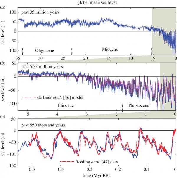
Take look at the graphs showing changes in sea level through the history of the Earth. The top figure covers 35 million years, the middle one covers a little more than 5 million years, and the bottom one zooms in to the past 500,000 years. What do you notice? Is there a regularity in the pattern of sea level ups and downs?
Through Earth’s history, there appears to have been a regular spacing of glacial maximum events, at roughly 120 thousand years (ky). When variations in Earth's orbit produce repetitive changes in climate and sea level, the observed cycles are often referred to as Milankovitch Cycles. Many sedimentary rock sequences have been shown to have stacking patterns that reflect these time scales, as do ice core data.

Milankovitch Cycles
Mathematician Milutin Milankovitch proposed an explanation for the changes in the way the Earth orbits the sun. These changes define the sequence of ice ages and warm periods.
- The Earth’s orbit changes from being nearly circular to slightly elliptical (eccentricity). This cycle is affected by other planets in the solar system and has a period of around 100,000 years.
- The angle of tilt of the Earth’s axis changes from 22.1° to 24.5° (obliquity). This cycle has a period of 41,000 years.
- The direction of the tilt of the axis changes (precession) on a cycle of 26,000 years.
- These changes influence the length of the seasons and the amount of solar radiation received by the Earth.
Optional Video
Please watch Milankovitch Cycles in 5 Minutes (5:00), if you are not already familiar.
[Music]
The Sun is the Earth's main energy source. In fact, it provides 99.96 percent of all the energy that drives the Earth's climate. Some of the energy produced by nuclear fusion in the sun's interior will eventually strike the top of the Earth's atmosphere. The amount of energy that does strike the atmosphere depends on two main factors: the total amount of energy produced and transmitted by the Sun, and the orbital cycles of the Earth with respect to the Sun. The energy transmitted by the Sun is in a constant state of flux depending on solar activities such as sunspots, solar flares, coronal loops, and coronal mass ejections. The relationship between the Earth's orbital cycles and climate change was proposed by Milutin Milankovitch.
Milankovitch was a Serbian engineer, and during the 1930s, he proposed that the changes in the intensity of solar irradiation received on the Earth were affected by three fundamental factors: precession, obliquity, and eccentricity. These factors are now collectively known as the Milankovitch cycles. The Milankovitch cycles are widely accepted by climate change scientists and are well documented by, for example, the IPCC. A more detailed description of the cycles is available by clicking on the tab above, but the remainder of this video will provide an excellent overview.
The Earth rotates on its axis every 24 hours. Around once in 27 days, the Sun also rotates on its axis. Its average distance from the Earth is approximately 150 million kilometers (93 million miles). It is an average distance because this Earth's orbit around the Sun is not fixed. Its orbit cycles from being almost a circle to that of an ellipse to almost a circle again. The cycle takes place over a period of around 100,000 years. The rotation of the Earth is at an angle to the vertical, and this angle changes over time. It moves from 22.1 degrees to 24.5 degrees and back again. This is over a time span of approximately 41,000 years. The Earth also goes through a cyclic wobble. It moves from its current position of the north pointing to the star Polaris to where the North points to the star Vega and returns to pointing at Polaris. The full cycle takes place between 19 to 26 thousand years. The combined effects caused the seasons to gradually cycle relative to the perihelion and aphelion, this over a time span of about 21 thousand years.
[Music]
How do these variations in Earth’s orbit affect climate and sea level? Collectively, variations in Earth's orbit (eccentricity, obliquity, and precession) can either reinforce signatures of cooling or warming, or they can work to counteract each other and produce less severe or ameliorated climate change. When the multiple variables reinforce each other, the amount of climate change and, as a result, sea level change can be significant.
Sea Level in the Past 20,000 Years
Sea Level in the Past 20,000 YearsIn order for us to connect sea level with our discussion on intrinsic and extrinsic controls and feedback mechanisms, etc., let's see another dataset that links climate history and sea level. The image below shows warm and cool periods for the last 900,000 years and has an expanded inset for the last 140,000 years.

In the inset, you will notice the long-term decline in sea levels from the last interglacial warm period, which occurred about 130 ky before the present. It is labeled stage 5e on the graphic. Sea levels declined to the lowest levels during stage 2 that occurred between 13,000 and 20,000 years ago. During this time, despite some minor short-term rise/fall events, sea levels fell from near modern sea levels to some 120 meters below present. The long-term rate of sea level fall calculation shows that sea levels fell 120 meters in approximately 100,000 years, or 0.12 m / 100 years. That is, sea levels fell by some 12 cm per 100 years, or through a simple unit conversion, the rate can be stated as 1.2 mm/year.
In the same graph, sea level rise appears to have been occurring at least for the last 18,000 years. Modern sea levels (relatively similar to highs 120,000 years ago) were achieved quite rapidly, relative to the rate of fall. Based on these numbers, 120 meters of sea level rise appears to have occurred in 18,000 years. This represents a rate of almost 6 mm/year for a rise rate.
This asymmetrical pattern of sea level rise/fall rates is repeated again and again for many of the earlier glacial-interglacial episodes. Thus, there is evidence that shows sea level fall (and building of ice sheets) is a long, drawn-out process where cooling and various positive feedback loops help to reinforce the cooling. The end result is an extended period of sea level fall (i.e., iteratively more albedo, and less and less insolation delivery, more cooling, etc.).
Conversely, once the factors that initiate warming begin to turn on, warming and associated sea level rise apparently can proceed at a much faster rate until a maximum sea level is reached, and factors that influence cooling initiate and bring sea levels down again.
Prior to the last few centuries, the system was controlled primarily by extrinsic and intrinsic variables. However, human impacts on landscapes, oceans, and climate (i.e., deforestation, greenhouse gas concentrations, nutrient runoff, aerosol pollution, and cloud development, etc.) have added variables that weren't present at any previous time (more on this later).
Now, let's look at a couple of more composite analyses that help us understand signals and signatures from the last few 1000 years. In the graphic below, a number of different datasets from Australia, South America, the Caribbean, the western Pacific, and other areas have been plotted to show sea level positions. Most of these datasets are derived from investigations of coral reefs that have drowned as sea level has risen.

From what is observed in the figure above, sea level rise rates appear to have been relatively low during the initiation of rise (i.e., from 20,000 to approximately 15,000 years ago), at which point a significant increase in sea level rise rates (Meltwater Pulse 1A), and several others ensued. Three rapid increases in rise rates ("pulses") are noted here so that the majority of the 100 meters of sea level rise occurred from 14,000 to approximately 8,000 years ago, or 90 meters in roughly 6,000 years. This yields a sea level rise rate of 0.015 meters per year or 1.5 centimeters per year or 15 mm per year.
This is an incredibly fast rate that is tied to the decay of large ice sheets, including both the Eurasian and Laurentide Ice Sheets. The Laurentide Ice Sheet on North America had mostly retreated from North America by 6,000 years ago, leaving behind only the alpine ice sheets. Check out the video below showing the retreat.
Video: Laurentide Ice Sheet (00:32) No audio.
Laurentide Ice Sheet
The Deglaciation of North America 21,400-1,000 years ago.
After Arthur S. Dyke, “An Outline of North American Deglaciation…” 2004. With additions from, “The Last Great Ice Sheets”, Denton & Huges, ed., 1981. Coastlines estimated using Barbados sea level curve after Bard et al., 1990. Great Basin Lakes from Curry, Atwood, and Mabey, “Map 73: Major Levels… Lake Bonneville” 1984.
[Animated map of North America shows the Laurentide Ice Sheet dramatically receding toward the northeast from 21,400 years ago, to 1,000 years ago.]
For more information
Check out Vignettes: Key Concepts in Geomorphology, for more info on Laurentide Ice sheet decay.
As these large ice sheets and their albedo potential were removed, the rate of absorbance of incoming solar radiation was likely to have contributed to further warming and increased temperatures of seawater. Thus, geoscientists are increasingly confident in the two primary factors that have contributed to the sea level rise rate prior to human influences. The primary cause is thought to be tied to thermal expansion of seawater, as we discussed previously. The second is the role of melting glaciers and increased volumes of land-ice being moved to the oceans.
Sea Level Change in the Holocene Epoch
Sea Level Change in the Holocene EpochIn the figure on the previous page, we observe that approximately 6,000 years ago, the rate of sea level rise slowed significantly. This left significant ice sheets on Greenland, Iceland, and Antarctica. Why didn't the rate of ice-sheet decay continue? That's a very good question. This time frame happens to coincide with decreasing incoming solar radiation values from Milankovitch forcing models.
Although it isn't yet clear, this relationship is a hypothesis that is being tested. Did the slowdown in the rate of sea level rise to a near still stand correlate to decreasing insolation in the Northern Hemisphere? Despite a level of greenhouse gas concentrations of ~265 parts per million, the rate of rise could not be sustained because the vast ice sheets were already melted and decreased insolation values per unit area in the Northern Hemisphere may have contributed to the development of stability in sea levels. In other words, greenhouse effects may have acted to continue to keep sea levels rising despite decreased insolation. Thus, sea levels achieved a much more stable condition.
For the period from roughly 6,000 years ago to the last century, the amount of rise is estimated to have been just a few meters. Hence, rise rates fell almost to zero (~0.7 mm/year), a far cry from the 15 mm/year rise rates estimated for the immediately preceding interval.
Under these relatively stable conditions, many of the coastal features observed today developed and expanded. Coral reefs that were able to keep up with earlier rates of sea level rise began to expand laterally, building large reef systems including the Great Barrier Reef and others in the Pacific Ocean, and the barrier reef systems common off south Florida and in the Caribbean. Likewise, deltas were built from sediments deposited by large river systems around the globe, including the Mississippi River delta. Numerous barrier islands were formed along the eastern seaboard and the Gulf of Mexico. They migrated slowly landward, up the continental shelf as sea level rose.

Recent Sea Level Rise and Anthropomorphic Impacts
Recent Sea Level Rise and Anthropomorphic ImpactsIn the human timeline, the change from higher rates of sea level to lower rates of sea level rise coincided with the onset of the Neolithic interval ~4,000 years ago. Although human beings began to influence Earth in interesting ways within the last few millennia, (think Roman Empire, which began to expand about 2,000 years ago), anthropogenic impacts on sea levels likely occurred more recently. Feedback loops often have significant lag times.
As human populations grew and the demand for freshwater for agriculture and other industries increased, and as forests were deforested, significant volumes of water re-entered the ocean-climate system and contribute to sea level rise. Some calculations suggest that perhaps as much as 5 percent of the sea level rise observed in the last few decades may be from these sources.
Recommended Reading
This National Geographic News article "Groundwater Depletion Accelerates Sea-Level Rise" is related to this topic.
In 2016, the Earth’s atmospheric carbon dioxide concentration reached the 400 parts per million threshold level. This was highly significant to climate scientists and all people concerned about the effects of climate change on the planet. The amount of CO2 in the atmosphere has increased from about 280 ppm since 1750 AD at the beginning of the Industrial Revolution to its current level of 420 ppm. This is significant because of the observed effect that these increased levels of, a powerful greenhouse gas, have on the warming of the atmosphere and in turn the ocean.
Climate scientists agree that this steady increase in carbon dioxide levels (as well as other greenhouse gases – water, methane, nitrous oxide) is the cause of the warming of the planet. The burning of fossil fuels by humans over the past few centuries has “unleashed vast reservoirs of fossil carbon stored in the Earth for hundreds of millions of years.” (Hearty). When the concentration of these compounds increases in the atmosphere, so to do global temperatures, as greenhouse gases limit the escape of long-wave radiation (thermal energy). These interactions result in a warmer climate, which means more glacial ice is being melted. When combined with more water released into the ocean, warmer ocean waters also expand in volume and result in higher sea levels.
If we look at the Earth’s history, it is extremely rare for Earth to have 400 ppm of carbon dioxide in its atmosphere. Paleoclimate research using ice core data shows that about 3 million years ago the atmosphere contained 400 ppm carbon dioxide. Then the sea levels were 10 – 40 m higher than today. In more recent Earth history, 800,000 years ago, during an interglacial period, there was 300 ppm CO2. As we discussed above, ice core data show that fluctuations in the Earth’s sea levels parallel atmospheric CO2 levels.
All this is evidence for the argument that as we continue to pour more CO2 into the atmosphere with continued fossil fuel energy reliance, we can expect sea temperatures and sea levels to continue to rise in tandem with the CO2 concentration. There are many other implications that go along with this scenario. We must remember the positive feedback mechanisms, such as that in which the melting of Arctic ice reduces the albedo effect – or the reflective nature of the white snow and ice. These types of mechanisms have the effect of accelerating warming and therefore increasing the melting of ice and, in turn, increasing sea levels.
Let’s look at the data from tide gauge records, graphed over the entire 20th century and into the 21st Century. The graph below represents a composite of 23 tide gauge records from around the globe for the last century (1880 to 2000), and altimetry data superimposed since 2000 (red line).

Each individual record shows the volatility (ups/downs) in water levels attributed to seasonal sea level changes that we have also previously discussed. To reduce this volatility, scientists employ a statistical averaging technique that calculates the average sea level of each successive three-year interval for all sites and then plots the average point on the graph. In this case, the moving average line is represented by the thick black line. Although it is still "wiggly," it is much smoother than the highly wiggly lines from which it is derived. This technique helps to "see the forest through the trees," so to speak.
Although a clear trend is visible in the 12 decades of data, the smoothed record helps to identify longer-term trends that are obscured by the highly variable local datasets. In this case, you will notice that there are essentially two modes in the longer-term trend. The first mode lasts roughly from 1880 through 1920, with a fairly stable sea level. In fact, the average sea level for this interval is used as the datum for this graph.
By 1920, the rate of sea level rise accelerates, and water levels begin to rise at a relatively constant rate through 2000 when satellite altimetry methods and data (red line) become available and help to substantiate tidal gauge methods.
These data show that sea level has risen an average of 20 cm (200 mm) over the last 80 years. This equates to a sea level rise rate of about 2.5 mm/year for the 80-year interval. If we take another look, including data collected since 2000, NOAA scientists show that the rate is accelerating again and a rate of 3.2 mm/yr. Has been established as the most current estimate.
The International Panel on Climate Change (IPCC) has set an estimated projected sea level rise at between 0.5 and 1.5 m by 2100. Many scientists argue that this is a too conservative estimate.
These estimates are based largely on the thermal expansion of seawater as the ocean surface heats up. However, the possibility of a significant contribution from the melting of ice sheets in Greenland and East and West Antarctic is not currently an important factor in IPCC predictions. Stay current as this research develops and estimates are adjusted accordingly.
Measuring Changes in the Arctic and Antarctic Ice Caps
Measuring Changes in the Arctic and Antarctic Ice CapsOne of the biggest uncertainties that has caused scientists to tend towards conservative estimates of sea level changes in recent years (and result in the frequent announcements of increased projections in the past few years) is the rate at which the Earth’s polar ice sheets are melting. In the 2007 IPCC report, the sea level rise projection agreed upon was a conservative 60 cm (~ 2 ft.). This number did not account for the possibility of rapid ice flow from Greenland or the Antarctic into the sea. These two ice sheets alone hold enough water to raise sea levels by 65 meters compared to 0.4 meters from all the world’s mountain glaciers. But, at that time, researchers felt that there was insufficient understanding of the ice sheets to be certain, so the IPCC resisted putting a number on it.
The most recent IPCC report (2013) increased this estimate to 98 cm or almost 1 meter.
This number has been bumped up further since 2014 with the most recent projections ranging from 0.2 to 2.0 meters (See NOAA Sea Level Rise viewer information in Module 4 Lab for more on these ranges).
Eliminating the uncertainty around quantifying the contribution of ice sheet melt-water to sea level increases is attributed to observations from NASA/German Aerospace Center’s twin Gravity Recovery and Climate Experiment (GRACE) satellites. These data indicate that between 2002 and 2016, Antarctica shed approximately 125 gigatons of ice per year, causing global sea level to rise by 0.35 millimeters per year.
In 2002, NASA launched the GRACE satellites, which track both ocean and ice mass by measuring changes in the Earth's gravitational field. The paired satellites orbit the Earth together and are spaced roughly 200 kilometers apart. Ice and water moving around the Earth exert different gravitational forces on the GRACE satellites. The satellites can sense the minuscule changes in the distance between one another caused by the change in gravitation force, which they measure and used to track water and ice mass change. It's thanks to GRACE that we know where the water flowing into the ocean came from. According to GRACE, melting of ice in Greenland increased sea level by 0.74 mm/year and melting in Antarctica by 0.25 mm/year since 2002. (Source: Smithsonian)
Recommended Resources
The science involved in understanding the behavior of ice sheets is growing rapidly. More data will no doubt be revealed in the upcoming years, which will help to increase the accuracy of sea level rise projections. Other work to measure the rate of change in the Antarctic is described in these NASA articles:
Modeling Sea Level Changes
Modeling Sea Level ChangesHow do the IPCC and other agencies arrive at these numbers: Current rate of sea level rise: 3.2 mm/ year (Source: NASA: Global Climate Change); Sea Level rise predictions: 0.2 – 2.0 meters rise by 2100 (NOAA)? The numbers, which are frequently adjusted and may vary according to the source, are achieved using modeling methods of different kinds.
Earth System Models integrate the interactions of atmosphere, ocean, land, ice, and biosphere to estimate the state of regional and global climate under a wide variety of conditions. They numerically model the atmosphere, oceans, land, and sea ice, and have biogeochemical components (for example, dynamic global vegetation models) to study the carbon cycle.
Earth System Models of Intermediate Complexity (EMICs)
Models of intermediate complexity bridge the gap between conceptual models with many simplifying assumptions, and extremely complex, three-dimensional models that attempt to include as many known processes as possible. (Source: NASA: Sea Level Change)
The data gathering by the many satellite missions described above is producing datasets that are used to populate the models. Modeling ocean and sea surface height is responsible for the creation of the incredible simulations seen in this module.
Although models can help tremendously in understanding complex interactions among components of Earth systems and their outcomes, they are never perfect, and all are given ranges of confidence due to uncertainty. They must be compared to observations to iron out their inherent errors. The challenges involved in modeling the contributions of the ice sheets to sea level rise have reduced the ability to provide a full picture of what is happening in the oceans. This area is a growing field, and we are likely to hear about breakthroughs in modeling these aspects of climate change in the near future. The figure below shows sea level curves based on the IPCC AR4 report, which estimates a sea level rise of 0.8 meters by 2100.
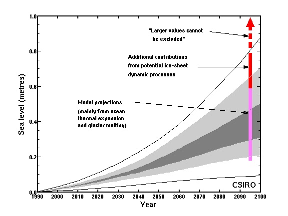
The figure above illustrates the levels of uncertainty that exist in the current data when using models to project future sea level rise. The AR4 IPCC data here show projected sea level curves through the year 2100. At 2095 the magenta bar shows a range of model projections (90% confidence limits), and the red bar shows the upper range extended to allow for the potential but poorly quantified additional contribution from a dynamic response of the Greenland and Antarctic ice sheets. Because there is a great deal of uncertainty surrounding the rates at which these ice sheets will melt in the future, a wide range of potential sea level rise scenarios are plotted. As the understanding of the mechanisms at work causing the melting of the ice sheets, the uncertainties shown here will most likely become more resolved in the future.
Summary and Final Tasks
Summary and Final TasksThe overall takeaways from the detailed discussions of sea level in this module are:
- sea levels are not uniform across the planet, so when we talk about mean sea level rise, these averaged numbers used tend to gloss over the fact that some places are experiencing greater or lesser effects, depending on many variables;
- the drivers of sea level changes over the history of the Earth are complex (including intrinsic and extrinsic factors) and feedback loops work to create cycles of sea level rise and fall, while maintaining an overall equilibrium;
- mean global (eustatic) sea level has been rising steadily during the 20th and early 21st Centuries;
- relative sea level rise causes large local differences in rates of sea level rise. Subsidence of the land can exaggerate sea level rise, while geologic uplift can cancel out some of the effects;
- the current rate of global sea level rise is quantified at 3.2 mm/ yr., a number which has increased in recent years, based on strong evidence that the rate of sea level rise is increasing;
- the chief driver for the acceleration in sea level rise in the past one hundred to two hundred years appears to be anthropomorphic in origin and caused by rapidly increasing atmospheric carbon dioxide levels due to fossil fuel combustion;
- paleoclimate research has established that sea levels have been much higher than today for much of the Earth’s history, with many factors at play, but atmospheric carbon dioxide levels appearing to be a chief driver in climate changes;
- glacial and interglacial periods during the past 500,000 years have been responsible for periods of rapid sea level rise, followed by periods of slower sea level fall as climate cools, glaciers form, and water is once again locked up in ice;
- the exact rates of increasing sea level depend on factors, such as rates of ice melt from polar ice caps, that are currently not understood well enough to give accurate projections;
- the Earth system science models are being refined continually, using more exact data from satellites, and will improve the ability of scientists to predict future sea levels;
- current projections for the end of the 21st Century are between 1 and 2 meters of sea level rise;
- a worst-case scenario suggests that if all the ice in Antarctica and the Arctic were to melt, there would result in a rise in sea level of 65 meters!
The implications of sea level rise – even the conservative projections – are huge for the millions of people around the world living in coastal communities. In Modules 5 and 6, we will consider how coastal catastrophes impact societies and how these societies are responding.
Reminder - Complete all of the Module 4 tasks!
You have reached the end of Module 4! Double-check the Module 4 Roadmap to make sure you have completed all of the activities listed there before you begin Module 5.
References and Further Reading
The following links are meant to provide suggestions for further investigation into the ever-changing landscape of sea level rise.
- Wikipedia: Sea level rise
- Smithsonian National Museum of Natural History: Sea Level Rise
- NASA: Understanding Sea Level - Causes
- NOAA - Climate Change: Global Sea Level
- NOAA National Centers for Environmental Information: What is Paleoclimatology?
- Climate Central: New Antarctic Research Ups Sea Level Rise Estimates
- NASA: NASA links port-city sea levels to regional ice melt
Module 4 Lab
Module 4 LabIntroduction
In this Lab, you will:
- Use the PSMSL website and Google Earth to explore historical records from tide gauges around the U.S. that provide reliable long-term data sets, to gain an understanding of different rates of sea level change on the Pacific, Atlantic, and Gulf coasts.
- Use NOAA's Sea Level Rise Viewer to make observations and compare sea level change predictions in locations around the U.S.
Lab Overview
There are two parts to this Lab.
- Part I is Analyzing Sea Level Change Using Tide Gauge Data. Download the tide gauge Google Earth KMZ data file from the PSMSL site. Use the tide gauge data to answer questions 1-14.
- Part II is the NOAA Sea Level Rise Viewer. After exploring and figuring out how to manipulate the viewer to give you the information for projected sea levels at the location of interest for different years, use the viewer to answer questions 9-15.
Part I: Analyzing Sea Level Change Using Tide Gauge Data
In Part I of this Lab, you will use data obtained from the Permanent Service for Mean Sea Level (PSMSL) in conjunction with Google Earth. A KML file is provided by PSMSL to open in Google Earth, making data access seamless. The sea level data are monthly and annual means referenced to a common benchmark and are referred to as a Revised Local Reference (RLR). This data is used to create accurate time series to observe trends. We are choosing four tide gauges with long time series. The longer the time series (more data), the more reliable the data are for looking at trends. You will notice short-term variability in the data – more in some locations than others. As you work through the lab, consider the difference between short-term and long-term time-series data and the reasons for the short-term variability that makes the data “noisy."
PART II: NOAA Sea Level Rise Viewer
Sea-level rise is expected to accelerate in the immediate future. However, even using the annual rates you calculated from the tide gauge data from the 20th Century and early 21st Century, a steady rise would be expected.
In Part II of this Lab, you will use the NOAA Sea Level Rise Viewer to help you visualize what these levels would look like in particular locations around the U.S.
You will keep your calculated rates in mind for each place from Part I, as you work with the viewer and consider the factors that influence the future projections of increased sea level rise.
NOAA built the viewer based on data that calculates a projected Global Mean Sea Level (GMSL) for 2100 to be between 0.3 m and 2.5 m. The model uses five GMSL rise scenarios: Intermediate-Low, Intermediate, Intermediate-High, High, and Extreme, which correspond to GMSL rise by 2100 of 0.5 m, 1.0 m, 1.5 m, 2.0 m, and 2.5 m, respectively (NOAA). For more detail on the science behind the Sea Level Rise Viewer, please take the time to read at least the Executive Summary and Introduction of NOAA Technical Report NOS CO-OPS 083 “Global and Regional Sea Level Rise Scenarios for the United States” listed in Resources.
Downloads/Resources
- Module 4 Lab Worksheet
- Tide Gauge KML File (see downloading directions below)
- Global and Regional Sea Level Rise Scenarios for the United States (Executive Summary and Introduction)
- NOAA Sea Level Rise Viewer Note: The viewer functions better if you use Google Chrome.
Directions for downloading tide gauge data using the PSMSL site and Google Earth
- Go to: PSMSL Tide Gauges.
- Follow the directions to download the tide gauge KML file and open it on Google Earth.
- The PSMSL RLR Catalogue folder will appear in your Temporary Places on Google Earth. Click on this folder to open, and select the Last Reported Year of 2018 or after (or the most recent available). This will reveal the tide gauges around the world with the most current data. These are the gauges we are interested in. We are also interested in those that have long and continuous datasets. We have chosen three with good data available, going back to early in the 20th Century. These are: Boston, MA, San Francisco, CA, and Grand Isle, LA. They also provide us with U.S. northeast coast, west coast, and Gulf Coast locations.
 Statement of Use of AI on Exams, Quizzes, and Labs
Instructions
Before you begin the Lab, download the Lab worksheet and tide gauge data. We advise you to either print or download/save the Lab worksheet, as it contains the steps you need to take to complete the Lab in Google Earth. In addition, it has prompts for questions that you should take note of (by writing down or typing in) as you work through the Lab.
Once you have worked through all of the steps and completed the measurements, you will go to Module 4 Lab (Quiz) to complete the Lab by answering multiple-choice questions. The answers to questions on this Lab worksheet will match the choices in the multiple-choice questions. Submit the quiz for credit.