Goals

On completing this module, students are expected to be able to:

• describe the processes that cause sea level to rise and fall;
• explain the evidence for sea level change in the geologic record and over the last century;
• project sea level rise in coming decades and beyond and their impact on coastal communities;
• propose strategies to cope with rising seas in communities that are most threatened by sea level rise.

Learning Outcomes

After completing this module, students should be able to answer the following questions:

• How much is sea level forecasted to rise in 2100?
• What are the processes that are causing modern sea level rise and what is the relative role of each?
• How much would sea level rise if all of the ice on Greenland and Antarctica were to melt?
• What is the current rate of sea level rise?
• What instruments are used to measure modern sea level rise?
• What faunas can be used to reconstruct ancient (but fairly recent) sea levels?
• When in the last 25 thousand years were the fastest rates of sea level rise?
• What are some of the processes that are causing relative sea level change in the region around New Orleans, and how much are some parts of the city subsiding?
• What do the terms transgression, regression, and sequence refer to and how do they fit into the concept of relative sea level change?
• What is reflection seismology and how does it help determine ancient sea level?
• Why was sea level so high in the Cretaceous and Eocene?
• What is storm surge, and why did it do so much damage during Katrina?
• What strategies are being used to prevent flooding in the next Katrina?
• What strategies are being used to prevent flooding on the Outer Banks, Netherlands, and Venice?
• What is the future of sea level rise in Bangladesh, Pacific Islands, and the Torres Straits?

Below is an overview of your assignments for this module. The list is intended to prepare you for the module and help you to plan your time.

Assignments

1. Lab 10:Impact of Sea Level Rise on Coastal Communities
2. Submit Module 10 Lab 1.
3. Take Module 10 Quiz.
4. Yellowdig Entry and Reply

For most people, sea level rise is caused by melting ice sheets. It is so easy to visualize a glacier melting into the ocean. As it turns out, an equally important factor is the expansion of seawater as it warms. In this section, we explore these different mechanisms in some detail.

Growth and Melting of Ice Sheets

How are absolute changes in sea level caused? As we have seen, the most direct way is through the growth and melting of the major ice sheets, as discussed in the following video.

Video: NASA: A Tour of the Cryosphere 2009 (5:12)

Iceberg Images

The following videos describe melting of ice sheets on Greenland and Antarctica.

Video: "CHASING ICE" captures largest glacier calving ever filmed (4:41)

Video: Antarctic Wilkins ice Shelf Collapse (No Narration) (2:20)

This process has been active over much of geologic time, all except for the very warmest time periods when there were no polar ice sheets. If we were to melt all of the ice on Antarctica and Greenland, we would see a sea level rise of almost 70 meters (Greenland would cause about 6 m of sea level rise, Antarctica about 60 m). This would take melting of the relatively stable interior of the ice sheets, which will take thousands of years to occur if modern warming rates continue unabated. However, there is much we do not understand about the behavior of the more dynamic areas of the ice sheets closer to the edges, and this imparts a great deal of uncertainty to any predictions of sea level rise in the coming centuries.

Crack recently exposed in the Pine Island Glacier, Antarctica, evidence that the glacier may soon break up. Other data suggests the glacier is being warmed from beneath by warm ocean currents.

Credit: NASA/GSFC/METI/ERSDAC/JAROS, and U.S./Japan ASTER Science Team

New research appears all the time that shows vulnerable parts of the Antarctic ice sheet, especially its shelves. Geologists are able to use radar instruments to image the base of the ice shelf and the seabed. Ice shelves refer to places where ice overlies seawater or bedrock that is below sea level. Recently, glaciologists have found places in West Antarctica where the underlying seabed is much smoother than expected, meaning that the glacier can advance readily under the right circumstances. Moreover, some of these places are vulnerable to being heated by warm ocean currents in the future. We presented the physical evidence for ice melting in Module 2, below are before and after photos from Alaska to remind you.

Muir Glacier in Alaska, as seen in 1941 and 2004

Photo courtesy of William Field (1941) and Bruce Molnia (2004) and the National Snow and Ice Data Center, University of Colorado, Boulder.

The second process that is causing sea level rise on human time scales is the physical expansion of seawater as a result of temperature increase. When materials are heated, they expand and, in the case of the oceans, this causes the surface of the water to rise. This thermal mechanism can cause absolute sea level changes on the order of millimeters and centimeters per decade. It varies geographically depending on how fast the ocean is warming in individual locations, and temporally depending on variations in ocean temperatures associated with climate oscillations such as El Niño . Hard as it is to imagine with all of the press attention over melting ice, but thermal expansion may actually cause more sea level rise in the 21st century.

The following video describes how satellites provide a very detailed picture of sea level change.

Video: How to Get NASA Sea Level Rise Data | Climate Analysis Tutorial (8:07)

In the past, the significant sea-level rise was caused by major episodes of volcanism that added crust in the ocean basins and displaced seawater towards land. This happened when processes deep in the interior of the earth caused seafloor spreading rates to increase and massive eruptions of volcanic submarine plateaus away from the ridge. These processes occur on very long or geological time scales and are not a factor today.

Scientists are increasingly concerned about one massive glacier, the Thwaites glacier, on the edge of the West Antarctic Ice Sheet. Satellite images show that the Florida-sized glacier is rapidly becoming destabilized, with giant cracks criss-crossing its surface. These features suggest that collapse could happen within the next decade. A large part of the Thwaites glacier on its eastern side is held back by a giant ice shelf, which is the part of the glacier floating on the ocean surface. The ice shelf acts as a brace or a buttress, holding the giant ice sheet back and keeping it from disintegrating. The ice shelf is being heated from below by the warming ocean and scientists have recently noticed cracks and crevasses, which signify that it is thinning. Moreover, these features allow warm water to attack further inside the glacier, accelerating its melting. At some stage, the ice shelf will break up, a phenomenon that is happening in numerous places along the edge of Antarctica. This will cause the Thwaites glacier to rapidly collapse into the ocean. Estimates are that this collapse would cause a 65 cm rise in global sea levels over a few years. Remember that sea levels are currently rising by millimeters per year and have risen by 20 cm since 1900, so this sudden rise would be unprecedented and catastrophic for low-lying cities such as New York, Miami, Mumbai, and Shanghai.

Melting of the Thwaites glacier already accounts for about 10% of global sea level rise. The glacier itself is also being attacked by warm water along its base. The ice grounding line, which is where the edge of the base of the ice sheet runs across bare continental rock, is being melted by warm waters pumped under the ice shelf by tides. This zone is rugged and chaotic with broken up rock, blocks of ice and warm water mixed in. As it melts, an ever thickening stack of ice is exposed to the warm water.

The collapse of the Thwaites glacier could also lead to failure of other nearby ice sheets via a process known as Marine Ice Cliff Instability. This is where rapidly retreating ice sheets that are un-buttressed by ice shelves, expose large, unstable cliffs that readily collapse into the ocean. So the collapse of Thwaites would expose the front of adjoining glaciers to the warming ocean, leading in turn to their collapse. Models suggest that the collapse of Thwaites could ultimately lead to the collapse of much of the Western Antarctic Ice Sheet, leading to three meters of sea level rise via this process. For this reason, the Thwaites glacier is also known as the “Doomsday Glacier”. The timing of its demise is currently impossible to predict, but the signs are that it is beginning to happen and the resulting sea level rise will have a very profound impact on coastal cities around the world.

The rapidly melting edge of the Thwaites Glacier

NASA, Public domain, via Wikimedia Commons

Video: Doomsday Glacier: Expers Raise Alarms About Cracking Antartctic Ice Shelf (7:08)

Sea level is rising at present and this rise provides some important insight into recent climate change — a warmer planet means the transfer of glacial ice to the oceans, and warming of the oceans causes an expansion of seawater. There are two main ways to directly measure recent changes in sea level — tide gauges and satellites. Tide gauges are fairly simple devices that record the height of sea level at a particular spot; the records are dominated by the daily tides (see photo below), but the data can be used to estimate the average sea level height each year.

Tide Gauges

Example of a tide gauging station from Anchorage, which has a huge tidal range.

Credit: NOAA

Tide gauges measure the height of sea level relative to the ground, and if the ground is stable, then they may be recording a global sea level change; if the ground is unstable, then the tide gauge record is difficult to interpret. Sites that are near the boundaries of tectonic plates are geologically unstable, so their tide gauge records are not reliable. Other sites located near the locations of formerly large ice sheets are also unstable in the sense that the land there is rising due to the removal of the ice from the last glacial age. This ice weighed a great deal (it was around 5 km thick) and its removal has triggered a very slow, steady rise of the crust — it’s like pushing down on a block of wood floating in the water and then removing your hand — the block rises up. Extending this analogy to the Earth, the block of wood is the crust and the water is the mantle, which is a very, very sluggish fluid, thus the crust does not spring up quickly, but takes several tens of thousands of years. If the land is rising up, then it would appear that sea level is falling, and indeed, this is seen in many tide gauge records from polar regions.

Tide gauge record from Churchill, Ontario (Canada), on the edge of Hudson’s Bay showing falling sea level.

Click for a text description of the Monthly Mean Sea Level graph.

The scatter plot shows monthly mean sea level data in millimeters from 1940 to 2010. The y-axis represents sea level in millimeters, ranging from 6600 to 7800 mm, while the x-axis shows years from 1940 to 2010. The data points, plotted as blue dots, exhibit significant variability but reveal a general downward trend over the 70-year period, starting around 7400 mm in 1940 and decreasing to approximately 6700 mm by 2010.

• Graph Overview
  • Title: Implied as Monthly Mean Sea Level (not explicitly stated)
  • Type: Scatter plot
  • Time Period: 1940 to 2010
• Axes
  • Y-axis: Monthly mean sea level (6600 to 7800 mm)
  • X-axis: Year (1940 to 2010)
• Data Points
  • Representation: Blue dots
  • Trend: General downward trend
  • 1940: Around 7400 mm
  • 2010: Around 6700 mm
• Variability
  • Description: Significant fluctuations throughout the period

Credit: Data from Permanent Service for Mean Sea Level (PSMSL)

This tide gauge record comes from Churchill, Ontario (Canada), on the edge of Hudson’s Bay; here, you can easily see the downward trend, meaning that sea level appears to be falling, but this is just in a relative sense. The story here is that the crust is rising, so sea level appears to be falling. The crust is rising in response to the melting of an ice sheet about 5 km thick that was present during the last ice age.

Because of the problem of crustal stability, tide gauge records have to be selected very carefully if we want to learn something about how global sea level is changing. Not surprisingly, this work has been done (Douglas, 1997), and a set of 23 tide gauge records have been selected, shown in the figure below.

This figure shows the change in annually averaged sea level from 23 tide gauges with long-term records (Douglas, 1997). The thick dark line is a three-year moving average of the tide gauges. The rise of sea level is not constant or simple, but the overall trend is fairly easy to see, indicating a rise of about 20 cm during this time period, at a rate that is about 2 mm/yr over the last 100 years. The red line shows changes in global sea level as measured by satellites, and you can see that there is very good agreement.

Credit: Data by Robert A. Rohde, figure created for Global Warming Art (CC BY-SA 3.0)

Satellites

The satellite data are interesting to consider — how can a satellite measure sea level changes? The answer is surprisingly simple at one level — it just measures the distance from the satellite to the sea level surface. The figure below shows how the system works, using a radar beam that bounces off the water surface and returns to the satellite. The height of sea level is actually the difference between the distance between the satellite and the sea surface and something called the reference ellipsoid, which is a kind of smoothed approximation of the Earth’s shape.

Schematic diagram showing how the TOPEX/POSEIDON satellite system monitors sea level height relative to the reference ellipsoid.

Click for a text description of the TOPEX/Poseidon Measurement System diagram.

The diagram illustrates how the TOPEX/Poseidon satellite measures ocean characteristics. The satellite, in orbit, uses a radar altimeter for ranging, a microwave measurement system for water vapor in the column, and communicates with a GPS satellite for positioning. It also interacts with a DORIS beacon and a laser ranging station on the ground. The diagram shows the sea surface, sea level, geoid, sea-floor topography, and a reference ellipsoid, with arrows indicating the measurement paths from the satellite to the ocean and ground stations.

• Diagram Overview
  • Title: TOPEX/Poseidon Measurement System
  • Type: Illustrative diagram of satellite measurement
• Satellite Components
  • Satellite: TOPEX/Poseidon
    • Position: In orbit
    • Features: Radar altimeter, microwave measurement system
  • GPS Satellite: Assists with positioning
• Measurement Methods
  • Radar Altimeter Ranging: Measures distance to sea surface
  • Microwave Measurement: Assesses water vapor column
  • Laser Ranging Station: Ground-based, interacts with satellite
  • DORIS Beacon: Ground-based, supports satellite positioning
• Ocean Features
  • Sea Surface: Top layer
  • Sea Level: Average height
  • Geoid: Gravitational surface
  • Sea-Floor Topography: Ocean floor structure
  • Reference Ellipsoid: Baseline for measurements
• Visual Elements
  • Arrows: Indicate measurement paths
  • Colors: Blue for ocean, beige for land, gray for stations

Credit: NASA

The satellite is orbiting the Earth at a height of around 1300 km and can cover the surface of the oceans in 10 days, making several hundreds of thousands of measurements during that time, and keeping very close track of where it is located relative to some control points on the Earth. As a result, this system can measure the mean sea level to within a few millimeters — quite a remarkable achievement.

The figure above shows the details of the satellite-based measure of sea level change, spanning just 18 years. There is a very regular annual variation of about 15 mm and then a more steady rise of about 50 mm over this 18 year period, giving us a rate of rise of about 2.8 mm/yr, which is somewhat higher than observed from the tide gauge data over the last 100 years.

Credit: David Bice © Penn State University is licensed under CC BY-NC-SA 4.0

These observations show that sea level is undoubtedly rising, but in a somewhat irregular pattern, and lead us to ask why. What is causing this rise in sea level? There are two main explanations for this rise. One is a simple expansion of seawater as it warms and becomes less salty — this is known as the steric effect. As seawater expands, it takes up a greater volume, and so the sea surface elevations rises. If the sea water warms by 1 °C, the steric sea level rise would be about 7 cm. An additional small increase comes from a slight freshening of the oceans — salty water is denser than fresh water. This steric effect is believed to account for the majority of the observed sea level rise. The other main reason for sea level rise is from the melting of glaciers, which transfers water previously stored above sea level back to the oceans. As we have seen, mountain glaciers around the globe are melting and so are the big ice sheets of Greenland and Antarctica.

The effect of warming and freshening of the oceans is believed to be behind the annual cycle seen in the above satellite data. As you might expect, the warming and freshening do not occur uniformly across the globe, so the global pattern of sea level rise and fall is somewhat complicated, and this goes a long way toward helping us understand why the tide gauge records (from the “stable” sites) show considerable variations.

Other Indicators

Looking further back, we must rely on the geologic record. Benthic foraminiferal species that live in marshes have narrow depth ranges. Foraminifera found in cores of tidal marsh sediments can yield the depth at which they live and dated to provide an age. In this way, geologists have determined changes in sea level of the North Carolina coastal zone back to 0 AD, before tidal gauges were employed. The curve shows a sharp increase in the rate of sea level rise in the middle of the 19th century, coincident with the Industrial Revolution.

Sea level change in North Carolina back to 0 AD obtained from benthic foraminifera in peat sediments.

Click for a text description of the North Carolina sea-level reconstruction graph.

The graph plots GIA-adjusted sea level in meters on the y-axis (-0.4 to 0.2 m) against years AD on the x-axis (0 to 2000). The graph includes data from Sand Point (gray) and Tump Point (blue) with error bands. It shows three distinct periods: a stable sea level from 0 to 855 AD (0 mm/yr), a slight rise from 855 to 1274 AD (+0.6 mm/yr), a stable period from 1274 to 1865 AD (-0.1 mm/yr), and a sharp increase from 1865 to 1892 AD (+2.1 mm/yr). Green change point indicators mark transitions at 855-1076 AD, 1274-1476 AD, and 1865-1892 AD.

• Graph Overview
  • Title: Summary of North Carolina sea-level reconstruction (1 and 2σ error bands)
  • Label: C
  • Type: Line graph with error bands
  • Time Period: 0 to 2000 AD
• Axes
  • Y-axis: GIA-adjusted sea level (-0.4 to 0.2 m)
  • X-axis: Year AD (0 to 2000)
• Data Sources
  • Sand Point: Gray error bands
  • Tump Point: Blue error bands
• Periods of Sea Level Change
  • 0-855 AD: Stable (0 mm/yr)
  • 855-1274 AD: Slight rise (+0.6 mm/yr)
  • 1274-1865 AD: Stable (-0.1 mm/yr)
  • 1865-1892 AD: Sharp increase (+2.1 mm/yr)
• Change Points
  • 855-1076 AD: Transition to rising sea level
  • 1274-1476 AD: Transition to stable sea level
  • 1865-1892 AD: Transition to sharp increase
  • Visual: Green peaks indicating change points

Credit: Figure from Kemp et al., Geology, v. 37, p 1035-8. Credit A. Kemp.

Corals provide a reliable way to determine sea level in the past since they grow within about 5 meters of the sea surface (see Module 7). If we find a coral submerged at 200 meters (see below), then sea level must have been 195-205 meters below current levels. In this way, sea level for the last 22 thousand years has been developed using the depths of corals, dated using carbon-14 or uranium isotopes, below current sea level.

This figure shows sea level rise since the end of the last glacial episode based on data from Fleming et al. 1998, Fleming 2000, & Milne et al. 2005, who collected data from various reports and adjusted them for subsequent vertical motions related to post-glacial rebound. Most of the data here come from radiocarbon dating of corals that are found below modern sea level — these particular corals are known to grow in water depths of just a few meters, so for them to be found at such depths below modern sea level requires that the ancient sea level was much lower.

Credit: Data by Robert A. Rohde, figure created for Global Warming Art (CC BY-SA 3.0)

Drowned Coral

Drowned coral reef from150 m water depth off Hawaii.

Credit: United States Geological Society

Besides coral, there are other indications of sea level rise. Fjords are drowned glacial valleys, and estuaries, such as the Chesapeake Bay, are drowned river valleys. Both of these morphological features indicate that sea level has risen recently.

Sea Level Rise

We can see that sea level changes much more dramatically on the timescale of the ice ages. The last ice age peaked around 20,000 years (20 kyr) ago, and at that time, a great deal of water from the oceans was locked away in large ice sheets, so sea level was about 120 m lower than it is today! This is a colossal change and it would have dramatically changed the coastlines of the world. It is interesting to consider the rate of sea level change associated with this transition out of the last ice age. Sea level rose by about 120 meters in about 10 kyr, giving us a rate of 12 mm/yr, which is about four times faster than the average rate of sea level rise today.

Imagine what the world looked like 20,000 years ago when sea level was so much lower. To help, look at the figure below, which shows the elevation both above and below current sea level. The modern shoreline is easy to see — it is where the green colors begin. The black line offshore shows about where the shoreline was when sea level was 120 meters lower than today.

Elevation map of part of North America showing the approximate position of the shoreline during the last glacial maximum, when sea level was about 120 meters lower than today due to the formation of large ice sheets.

Credit: David Bice © Penn State University is licensed under CC BY-NC-SA 4.0

Now, more realistically, let's imagine what will happen to the coastal zone in coming centuries if sea level rise accelerates. We will observe flood maps in the following lab.

In fact, changes in the height of the ocean as a result of melting ice or warming seas (absolute or eustatic sea level change) only tell part of the story. The level of the ocean can also change because the underlying land is rising or falling with respect to the ocean surface. Such relative sea level change usually affects a local or regional area, and in numerous cases, is actually outpacing the rate of sea level change.

Relative sea level changes can be caused by plate tectonic forces. For example, the Great Japan earthquake on March 11, 2011, caused part of the island of Honshu to rise up by nearly three meters. The sea floor can also drop when huge amounts of sediment are deposited by rivers and deltas. The weight of the sediment depresses the underlying crust, often at a faster rate than the sediment is being deposited. This process is happening along the east coast of the US today in places along the coasts of Maryland, North Carolina and Georgia, and the Gulf Coast, especially in the Mississippi Delta region. In parts of Florida where large amounts of water have been pumped out of aquifers for water supply, the land is also subsiding rapidly.

Relative

One of the most drastic examples of relative sea level change is around New Orleans, where sea level is rising with respect to the land at alarming rates. The map below left shows that in parts of the city, the land surface is subsiding at nearly 3 cm per year! There are two additional alarming parts of this story. The first is that the rates actually may have been faster in the past and have the potential to increase again; the second is that parts of the city already lie 4 meters below sea level (see map below left). The causes of the New Orleans subsidence are partially natural. The city sits on delta sediments that are accumulating very rapidly and causing the underlying crust to subside due to their weight. However, humans are also responsible. Draining wetlands, over pumping aquifers and diverting floodwaters from the Mississippi River are all contributing to rapid subsidence.

The New Orleans subsidence map is an excellent example of relative sea level change. However, the fact that the land the city is built upon is subsiding so rapidly makes it more prone than most areas to absolute sea level rise as a result of warming oceans and melting ice sheet. Late in this module, we will observe some of the changes the city has made to combat both sources of sea level rise. However, the rates of subsidence are so rapid that some scientists are advising retreat from the coast as the wisest option from an economic and safety point of view.

New Orleans Flooding Maps

Diagram showing the changes that can lead to relative rise of sea level (or transgression) and relative fall in sea level (regression).

Click for a text description of the Sea Level rise and fall diagram.

The diagrams illustrating coastal changes due to sea level fluctuations. The top diagram shows a transgression phase where the shore migrates inland, with the shoreline moving over land due to rising sea levels, depicted with a blue ocean layer encroaching onto a green and brown landscape. The bottom diagram illustrates a regression phase, labeled "maximum limit of transgression," where the shore migrates seaward due to falling sea levels, exposing more land. It highlights uplift and erosion with a yellow arrow, showing sediment layers and a river system forming as the ocean (blue) retreats from the land (green and brown).

• Diagram Overview
  • Type: Two cross-sectional views of coastal changes
• Top Diagram (Transgression)
  • Description: Shore migrates inland
  • Visual: Blue ocean layer encroaching on green and brown land
  • Label: Shore migration inland
• Bottom Diagram (Regression)
  • Description: Shore migrates seaward
  • Labels: Maximum limit of transgression, shore migration seaward
  • Visual: Blue ocean retreating, exposing green and brown land
  • Additional Process: Uplift and erosion
    • Visual: Yellow arrow indicating uplift and sediment layers
  • Features: River system forming on exposed land

 

Credit: Stephen Marshak

Once this regression reaches a certain point, much of the shelf becomes subaerial and characterized by sporadic deposition and erosion. This erosion makes a surface that is called an unconformity, which is essentially a gap in time. The unconformities end up bounding a package of strata that is deposited by one individual sea level rise and fall. Such packages are known as sequences. The multiple sea level rises and falls have produced sequence upon sequence underneath the continental shelf and slope. These sequences hold within them the history of relative and absolute sea level change.

Geometry of sequences showing the different types of sediment. Land is located to the left, ocean to the right.

Click for a text description of the Complete depositional sequence image.

The diagram Illustrates a cross-sectional view of layered sediment deposits. It shows various systems tracts labeled TST, HST, FSST, and LST, representing different phases of sediment deposition. The layers are color-coded: green for coastal plain, yellow for shallow-marine sandstone, and gray for offshore mudstone with subaerial erosion and exposure. A note indicates that not all systems tracts are present at any given location. Red lines mark the boundaries between the tracts.

• Diagram Overview
  • Title: Complete depositional sequence
  • Type: Cross-sectional view of sediment layers
• Systems Tracts
  • TST (Transgressive Systems Tract)
  • HST (Highstand Systems Tract)
  • FSST (Falling Stage Systems Tract)
  • LST (Lowstand Systems Tract)
  • Visual: Labeled with red boundary lines
• Layer Types
  • Coastal Plain
    • Color: Green
  • Shallow-Marine Sandstone
    • Color: Yellow
  • Offshore Mudstone and Subaerial Erosion and Exposure
    • Color: Gray
• Additional Note
  • Text: Not all systems tracts present at any given location

Credit: Steven Holland, University of Georgia, Online Guide to Sequence Stratigraphy

Geophysicists can image the subsurface using a technique called reflection seismology. Basically, elastic waves from ships are produced by airguns, these waves travel down through the ocean and reflect back off the seafloor and the layers underneath it. It turns out that the unconformities between the sequences reflect a lot more energy than the conformable layers within the sequences, so the sequences can be mapped precisely using reflection seismology. Individual sequences can be age dated using microfossils (see Module 1) and in this way, the history of sea level can be determined. This technique is known as sequence stratigraphy.

Absolute

So, the big question is how we know whether sequence stratigraphy reflects relative sea-level change caused by changes in subsidence, sedimentation, and sediment loading, as we discussed in the previous section, or absolute or eustatic sea level changes? The way individual sequences can be confirmed as eustatic is when they are observed on different continental margins (it would be difficult to imagine how regional subsidence, sedimentation patterns, and sediment loading would impact margins in a different part of the world at the same time).

Absolute sea level changes (in meters) over the last 540 million years. Present sea level is zero meters. The blue curve is from Exxon; red curve is from Hallam.

Click for a text description of the Global Sea Level Fluctuations graph.

The graph shows sea level changes in meters on the y-axis (-150 to 400 m) over millions of years ago on the x-axis (0 to 542 million years). The graph features two data sets: a red line labeled "Hallam et al." and a blue line labeled "Exxon Sea Level Curve." Both lines fluctuate significantly, indicating sea level rises and falls across geological periods marked on the x-axis: Neogene (N), Paleogene (Pg), Cretaceous (K), Jurassic (J), Triassic (Tr), Permian (P), Carboniferous (C), Devonian (D), Silurian (S), Ordovician (O), and Cambrian (Cm). A notable drop occurs during the Last Glacial period, around 0-50 million years ago, with sea levels falling to around -100 m.

• Graph Overview
  • Title: Global Sea Level Fluctuations
  • Type: Line graph
  • Time Period: 0 to 542 million years ago
• Axes
  • Y-axis: Sea level change (-150 to 400 m)
  • X-axis: Millions of years ago (0 to 542)
• Data Sets
  • Hallam et al.: Red line
  • Exxon Sea Level Curve: Blue line
• Geological Periods
  • Neogene (N), Paleogene (Pg), Cretaceous (K), Jurassic (J), Triassic (Tr), Permian (P), Carboniferous (C), Devonian (D), Silurian (S), Ordovician (O), Cambrian (Cm)
• Key Event
  • Last Glacial: Around 0-50 million years ago
    • Sea Level: Drops to around -100 m
• Trend
  • Description: Both lines show significant fluctuations, with peaks and troughs across periods

Credit: Data by Robert A. Rohde, figure created for Global Warming Art (CC BY-SA 3.0)

As it turns out, sea level curves such as the ExxonMobil curve have a hierarchy of cycles. Very short frequency cycles with frequencies lasting a few thousand years are superimposed on cycles with millions of year frequencies, and these are superimposed on long frequency cycles lasting 100s of millions of years. The current chart has five orders of cycles, all superimposed. The longer order cycles are almost certainly eustatic in origin. The shorter order cycles which cannot unequivocally be matched between continents are likely relative sea level changes. The big argument is whether the cycles in between represent absolute or relative sea level changes. Long order changes likely represent slow processes such as changes in seafloor spreading, whereas middle order cycles likely represent faster sea level changes associated with melting of glaciers.

We have been there before. There is plentiful evidence that the sea flooded the interior of continents multiple times in Earth history. These marine incursions alternated with times when the ocean receded to below the level of the current continental shelf. The sedimentary rocks that are found in the interiors of continents contain the fossilized remains of marine organisms such as clams, oysters, and corals, demonstrating that they were deposited below the sea. Geologists have known about these continent-scale sea level fluctuations for a long time. In the 1950s and 1960s, the brilliant geologist Larry Sloss of Northwestern University mapped out marine units across from one side of North America to the other and showed that they lasted many millions of years.

Map of the US about 90 million years ago with a seaway that flooded the central part of the continent.

Credit: William A. Cobban and Kevin C. McKinney, USGS (Public Domain)

We now know that some of the highest sea levels took place at times when the climate was warm and there were no ice sheets covering the poles. Likewise, times when global sea level very low corresponded to cold intervals when the ice sheets were extensive. As we established in Module 5, one of the main drivers of climate during these times was the amount of CO₂ in the atmosphere.

One period with high CO₂ levels, the late part of the Cretaceous about 90 million years ago, was a time when the high latitudes were too balmy to maintain ice sheets. There is much evidence for late Cretaceous warmth, none less compelling than the discovery of fossils of palm trees and reptiles in northerly places such as Alaska and Ellesmere Island in northern Canada. Beginning in the late Eocene (about 40 million years ago) ice began to accumulate on Antarctica and in the late Pliocene (about 3 million years ago) the northern hemisphere ice sheets began to grow. These changes in the psychrosphere (the technical name for the major ice sheets) led to substantial changes in sea level. In fact, some estimates of sea level in the middle Cretaceous are 170 meters higher than at present and those in the Eocene are 100-150 meters higher (see curve below).

Absolute sea level changes (in meters) over the last 540 million years. Present sea level is zero meters. The blue curve is from Exxon; red curve is from Hallam.

Click for a text description of the Global Sea Level Fluctuations graph.

The graph shows sea level changes in meters on the y-axis (-150 to 400 m) over millions of years ago on the x-axis (0 to 542 million years). The graph features two data sets: a red line labeled "Hallam et al." and a blue line labeled "Exxon Sea Level Curve." Both lines fluctuate significantly, indicating sea level rises and falls across geological periods marked on the x-axis: Neogene (N), Paleogene (Pg), Cretaceous (K), Jurassic (J), Triassic (Tr), Permian (P), Carboniferous (C), Devonian (D), Silurian (S), Ordovician (O), and Cambrian (Cm). A notable drop occurs during the Last Glacial period, around 0-50 million years ago, with sea levels falling to around -100 m.

• Graph Overview
  • Title: Global Sea Level Fluctuations
  • Type: Line graph
  • Time Period: 0 to 542 million years ago
• Axes
  • Y-axis: Sea level change (-150 to 400 m)
  • X-axis: Millions of years ago (0 to 542)
• Data Sets
  • Hallam et al.: Red line
  • Exxon Sea Level Curve: Blue line
• Geological Periods
  • Neogene (N), Paleogene (Pg), Cretaceous (K), Jurassic (J), Triassic (Tr), Permian (P), Carboniferous (C), Devonian (D), Silurian (S), Ordovician (O), Cambrian (Cm)
• Key Event
  • Last Glacial: Around 0-50 million years ago
    • Sea Level: Drops to around -100 m
• Trend
  • Description: Both lines show significant fluctuations, with peaks and troughs across periods

Credit: Data by Robert A. Rohde, figure created for Global Warming Art (CC BY-SA 3.0)

We have seen that if we melt all the ice on the Antarctic and Greenland ice sheets, that sea level will rise by about 70 meters. So how come sea level in the Cretaceous and Eocene was almost double this amount higher than at present?

The answer to this question is not just a climatic one. The Cretaceous, in particular, was a time of very active volcanism. Thick deposits of volcanic ash are found in Cretaceous marine sediment sequences, suggesting some gargantuan volcanic eruptions. Moreover, there is substantial evidence that volcanic activity was also more intense in the ocean basins themselves. Numerous large plateaus, known as large igneous provinces, or LIPS for short, date back to the Cretaceous. One of these, the Ontong Java Plateau in the western Pacific, is an area as large as Alaska and up to 30 km thick. In total, the Ontong Java eruptions lasted a few millions of years and spewed out 100 million cubic kilometers of lava. The period from 125 to 90 million years ago was characterized by very active volcanism. In addition to the Ontong Java Plateau, there are numerous other LIPS in the Pacific and Indian Oceans, as well as the Caribbean. In fact, much of the western part of the Pacific Ocean is characterized by a topographically elevated crust of Cretaceous age, known as the Darwin Rise, that was produced during times of very active volcanism. The Darwin rise is peppered with volcanic islands and seamounts.

Location of Large Igneous Provinces or LIPs

Credit: Millard Coffin

There is evidence that the largest of the LIP eruptions including the Ontong Java Plateau and the Caribbean involved the outgassing of so much CO₂ that they caused abrupt global warming events somewhat similar to the PETM. Because the ocean was already quite warm at these times, and warm water can hold less oxygen than cold water (as we saw in the section on hypoxia in Module 6), the Cretaceous LIP eruptions are thought to have triggered ocean wide hypoxic or anoxic events that led to the deposition of sediments called black shales. As it turns out, these black shales are thought to have sourced large amounts of the world’s petroleum, and the hypoxic events had major evolutionary consequences.

Black shale of Jurassic age at the base of a quarry in Humberside, UK.

Credit: Tim Bralower © Penn State University is licensed under CC BY-NC-SA 4.0

Emplacement of LIPs would have displaced a lot of seawater in the oceans. Thus, this volcanism can explain why sea level was significantly higher than the modern ocean, even with the complete melting of the ice sheets. The other potential reason is that the Cretaceous also saw higher rates of volcanism at mid-ocean ridges, which would also have displaced seawater and elevated sea level.

In this section we explore current and future challenges posed by sea level rise. Our example case studies come from the developed and developing world. We will see that there will be a very different range of options in countries with ample resources from those without.

Let us assume that by 2100 sea level will rise by amounts similar to the upper bounds of the 2007 IPCC estimates, roughly 60 cm. At the same time, let's assume that subsidence rates on the New Orleans region continue at current rates between 2 and 28 mm/year. The result would be between 0.8 and 3.1m of sea level rise relative to the current land surface.

Even if sea level rise does not inundate low-lying coastal regions, it will make them more prone to flooding during storms and prolonged periods of heavy rainfall. In fact, this is the predominant fear in places like Bangladesh and the Mississippi Delta region near New Orleans. Let's consider the area around New Orleans where hurricanes are a constant threat. The extensive damage caused by Hurricane Katrina did not arise from wind or rain, rather the massive storm surge, the giant wall of water that was pushed up onto the land during the hurricane. This storm surge was over 9 meters to the northeast of the city and peaked at about 5 meters within the city limits. This water either overtopped the levees and flood walls that were built to protect low-lying areas of the city, or, more frequently, combined with the wave action to topple levees from the base upwards. In the aftermath of Katrina, the Army Corps of Engineers has rebuilt the levee and floodwall system in New Orleans, and upgraded pump stations, to defend the city from a similar storm surge in the future. The new system offers multiple lines of defense beginning outside of the perimeter of the city. The massive Inner Harbor Navigation Canal Lake Borgne Surge Barrier is the largest flooding structure in the US.

Levees

The following videos describe how subsidence is leading to sea level rise in the Mississippi Delta region and how engineering is being used to combat it.

Video: Sea-Level Rise, Subsidence, and Wetland Loss (9:44)

Video: New Orleans Levees (2:07)

The design of all of the New Orleans flood protection is based on the elevation of a flood that occurs every 100 years. In other words, there is a 1% chance that the system will fail each year. You might ask why this risk is being taken and the structures have not been built higher. The answer is that it costs a large amount of money to build of the structures to withstand higher water levels.

Although New Orleans has received much attention after Katrina, and rightly so, many other areas are also at great risk from hurricane winds, waves and storm surge.

Outer Banks, North Carolina

One of the most popular holiday spots on the East Coast, the Outer Banks (OBX) of North Carolina, is also highly susceptible to sea level rise. In fact, recent research suggests that the OBX may be experiencing some of the fastest sea level rise on the planet at least as a result of very rapid subsidence of the land. Sea levels in OBX have climbed as much as 3.7 centimeters (1.5 inches) per decade since 1980, while globally they've risen up to 1.0 cm (0.4 inches). Models suggest that sea level may rise by up to 1.6 meters (5 ft) by 2100! The Outer Banks are part of a chain of barrier islands that stretch from Florida to Massachusetts along the Atlantic seaboard. Barrier Islands are delicate sand bodies that are generally moving towards the adjacent continent as sea level rises; this process occurs largely because storms erode sand from the seaward side of the island and deposit it on the landward side. The OBX is moving at a rate that is quite alarming from a development point of view, a point illustrated best by the famous Cape Hatteras lighthouse. The lighthouse was built in 1870 some 1,500 feet from the ocean. By 1970, the lighthouse was just 120 feet from the ocean, and its fate was not very uncertain. Fortunately, the lighthouse was moved some 2900 feet inland. At the rate the OBX are shifting, all development is threatened. However, development modifies the response of the coastal environment to erosion from storms often increasing erosion rates along the undeveloped parts of the coastline.

The OBX are extremely vulnerable to storms as a result of their exposed position in the open Atlantic Ocean, which has led to a greater number of hurricanes. As we have seen, experts predict there will be fewer more powerful storms in the future. The impact of these storms will be amplified by the continuing sea level rise and a powerful hurricane could have an extremely destructive impact on the fragile barrier islands.

North Carolina Storm Damage

One of the most vulnerable places for sea level rise in the US if not the world is Miami and more specifically Miami Beach, which lies on a fragile barrier island along the coast. Miami has a booming tourism and real estate industry, and Miami Beach and other beachside communities house some of the most luxurious developments in the country. According to Zillow, Miami contains 26 percent of homes at risk of rising seas. Sea level in the area is rising at a rapid rate, with six to ten inches of rise expected by 2030 and up to six feet by 2100. This is threatening everything. Six feet of rise would leave much of Miami Beach (and the Greater Miami area) underwater. Even six inches could be more damaging during hurricanes with storms surge pushing further inland and causing more destruction, but six feet would be truly devastating during these events. Left unchecked, the city could lose its thriving economy and be faced with massive damages from the rising waters within a couple of decades.

The last decade in Miami Beach has seen a dramatic increase in “sunny day” flooding events, which generally occur at monthly high tides, and some more drastic “king tide” flooding during the highest tides of the year. All of these events have led to flooded streets and parking lots. Rising seas also threaten Miami’s drinking water as salt water is beginning to seep into the city’s aquifer, threatening its water supply (the salt water incursion issue discussed in Module 8). Sea level rise also has the potential to destroy many of the city’s septic systems.

October 17, 2016 tidal flooding on a sunny day, during the "king tides" in Brickell, Miami that peaked at 4 ft MLLW.

Credit: Image by B137 from Wikipedia, licensed under CC BY-SA 4.0

Film crew in Miami Beach, sunny day high tide flooding

Credit: Maxstrz from Flickr (CC BY 2.0)

Miami Beach high tide flooding

Credit: B137 (CC BY-SA 4.0)

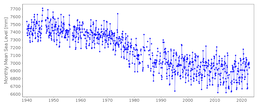
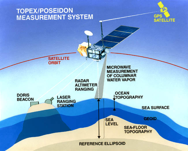
Faced with these threats, the city managers have taken on extremely proactive measures to stave off the rising seas and give the city a future. The city has raised taxes and employed some of the top coastal engineers to design systems to hold back the rising ocean. These systems include elevating the roads and building walls to protect key structures. Powerful pumps are being installed to drain water away during the king and sunny day high tides. Valves are being placed in drinking water systems to keep salt water out of the drinking water supply.

All of these measures are designed to ensure that the city stays vibrant well into the future even when the rate of sea level rise increases.

Video: Is Miami Beach Doomed? (6:28)

Venice

Next, let's travel to Venice. The average rate of land subsidence is about 1mm/year, largely due to the consolidation of the sediment and pumping of aquifers. This low amount is at odds with reports of crumbling building foundations and regular flooding of city monuments. What is going on?

Flooding in Venice

Venice has a long legacy of devastating flooding and the severe threat of sea level rise rendering the historic city uninhabitable, and, potentially destroying art and architectural treasures and spoiling a major tourism industry. Today, the average elevation of Venice is close to sea level. The city lies in a location with a moderate (certainly not large) tidal range of less than one meter. Yet, high tides regularly cause flooding. In fact, flooding driven by high tides submerges the lowest 14 percent of the city four times a year. The situation is where it is today in part because the land the city is built upon is rapidly subsiding due largely to the removal of groundwater. The city subsided 12 centimeters in the two decades before 1970. The old buildings are constructed on wooden pilings that sink into the mud, making them even more susceptible to subsidence. With so much at stake, the city is fighting back. Construction is well underway in the MOSE (Modulo Sperimentale Elettromeccanico, Experimental Electromechanical Module) project to construct giant barricades to keep floodwater from the Adriatic Sea out of the city. The flood control system will consist of 78 giant barriers that will rise out of the water when floodwaters threaten and prevent water from entering the three entry points to the lagoon. The barriers are like giant airbags inflated by air that fills in response to the water level. Once the threat passes, the barriers will fill with water and be lowered back to the seabed. The project has suffered numerous delays and there is growing frustration that it will be too little too late when it is completed, hopefully in 2021. Meanwhile, the floods continue.

MOSE Project

Holland

The Netherlands is an extremely low-lying country, about a quarter of which lies below sea level and half of which is within a meter of sea level. The city of Rotterdam, Europe’s busiest port lies below sea level. Two-thirds of the country is vulnerable to flooding from the sea and from rivers. Even before the threat of sea level rise came on the horizon, the country had already invested a great deal in engineering projects to keep the sea at bay. Like New Orleans and Katrina, the Dutch had their own “wake-up” call in 1953 when a high-tide storm breached levees, flooded a massive area and killed 1900 people. The country responded by developing a major flood control enterprise, the most extensive storm protection system in the world. Currently, the land is protected by a massive system of human-constructed levees, storm-surge barriers, dunes, canals, pumping stations and floodgates that are emplaced when tides are abnormally high or storms threaten. The system is designed to survive flood levels that occur only every 10,000 years (note the new levee system in New Orleans is designed to withstand the 100 year flood), however with rising sea levels and the potential for increased storm activity, the Dutch are looking to increase their efforts to keep the sea at bay. They plan to invest over $2 billion per year for the next 100 years to change drainage patterns to relieve the current strain on certain canals, in part by flooding land that is dry today. The scheme also proposed to reclaim more land from the ocean and push the shoreline out to sea. Moreover, the Dutch are even mulling building construction of floating cities. With decades worth of engineering experience, countries that are threatened by rising seas are looking to the Dutch for advice and innovation.

Holland

The following video provides an overview of engineering in the Netherlands designed to combat sea level rise.

Video: Oosterschelde Storm Surge Barrier - Virtual Tour. This video is not narrated. (4:45)

Bangladesh

Finally, let's visit the country of Bangladesh, where a large swath of the populous coastal lies very close to sea level. In fact, a one-meter rise in sea level would inundate 30,000 km2 and displace 20 million people. This area is already extremely prone to flooding from cyclones, and this danger will increase with sea level rise.

Bangladesh Flooding

The following video provides a stark picture of flooding in Bangladesh in 2004.

Video: Complete Bangladesh Movie (3:33). This video is not narrated.

Pacific Islands

A dire picture also emerges in small island nations in the western Pacific, including Kiribati, Tuvalu and the Marshall Islands, where sea level rise over the next century could cause these nations to completely disappear. In fact, the President of the nation of Kiribati has publicly stated that the 100,000 citizens in his country may need to be relocated as a result of climate change and sea level rise. In Tuvalu, large tides occurring in January, February, and March, and August, September, and October, known as King Tides, flood some areas of the main island and capital city Funafuti. Before sea level rise was a problem, these tides did not cause extensive flooding. Now, they are responsible for salinization of the soil which makes it infertile and for spreading diseases because of the leaking septic tanks, as well as loss of inhabitable land.

Like in the Torres Straits, inhabitants on many low-level islands in the Pacific are building sea walls to keep the rising seas out. However, in many places, the walls are built out of coral, often obtained from fragile offshore reefs that themselves offer some protection from the rising seas.

Pacific Islands

Torres Strait

One hundred and fifty islands lie between Cape York Australia and Papua New Guinea, 17 of the islands are permanently inhabited by about 7000 people belonging to indigenous populations related to the Aboriginal peoples of mainland Australia. With an average elevation close to sea level and a large tidal range (spring tide is about 10 feet), the islands are very prone to the effects of sea level rise. Trends suggest that the island may be characterized by a slightly higher rate of sea level rise than the global average. Even if the islands remain emergent, as sea level rises, they will still be far more prone to the impact of extreme events such as tropical cyclones as well as regular high tides. With very limited resources, the islands have had a piecemeal response to rising sea levels by building sea walls along the low-lying area. Unfortunately, these walls are in dire need of repair and reinforcement. Torres Islanders have pleaded with the Australian government to help rebuild and fortify the sea walls to protect the vulnerable areas. In August 2011, the government appropriated $22 million to build the wall, however, they backtracked four months later and, thus, the plight of the islanders remains in jeopardy.

Torres Strait

So, a final word. As you can imagine, Hurricane Sandy has reinvigorated the call for flood barriers and sea walls at the entrance to the New York City harbor. Such structures are very expensive, but would have saved an enormous amount of destruction from the storm. This is not the only city where flood barriers will be needed in the future, as the video below describes graphically.

Video: RockWorks: EarthApps - Sea Level Rise Simulations (3:01)

Download this lab as a Word document: Lab 10: Impact of Sea Level Rise on Coastal Communities (Please download required files below.)

There are two parts of this lab. In the first, you will look at recent trends in sea level from tidal gauge data going back to about 1940. This will allow you to determine the places where sea level is rising the fastest. In the second part of the lab, you will be looking at future sea level rise projections for certain areas. The first part of the lab is in Google Earth; the second part is in a web browser (the Google Earth files for this type of analysis don’t work well yet).

Files to Download

PSMSL Tide gauge file

Practice Questions

Part 1.

In this part of the lab, you will look at tide gauge data showing relative sea level rise data back to about 1940. The goal will be to determine trends from rather noisy data, determine places where relative sea level is rising faster than others, and the reason for the rapid rise. In the practice lab, we will focus on the West Coast of the US.

Load the PSMSL Tide gauge file in Google Earth. The file shows tide gauge data from around the world, which will allow you to explore the rates of sea level rise. The dots show stations organized by the last reported year. Click on stations, and you will see a PSMSL ID number; click on that, and you will get tidal gauge data in mm (for several locations, several dots appear; make sure you click on one of the dark green dots).

1. Go to Crescent city in Northern California. Is relative sea level rising or falling over time?
   1. Rising
   2. Falling
2. Roughly how much has relative sea level changed since the beginning of the record at Cresent City?
   1. Over a meter
   2. Over 0.25 m
   3. Under 0.25 m
3. Now go to Neah Bay in Washington State in the tip of the Olympic Peninsula. Is relative sea level rising or falling over time?
   1. Rising
   2. Falling
4. Roughly how much has relative sea level changed since the beginning of the record at Neah Bay?
   1. About 0.5 m
   2. About 0.3 m
   3. About 0.1 m
5. Based on just these two records, what is the dominant process controlling relative sea level change in these locations?
   1. Isostatic rebound (removal of ice)
   2. Subsidence
   3. Uplift due to tectonic activity

Part 2.

Prediction of the extent of flooding that results from sea level rise is much simpler than predicting the absolute amount of sea level rise that will occur over coming decades. Flooding predictions are based on digital elevation maps that have great accuracy and resolution. The NOAA sea level rise and coastal flooding tool allows you to look at areas in detail and make predictions about the future under higher seas. At the top, you can enter an address to look closely at an area. For the practice, we will look at Tampa, FL, so enter this in the search window. Note: it can take a while for a clear image to come into view. Remember 1000 mm is a meter.

Go to NOAA Sea Level Rise Viewer and click on Get Started. You will see a map focused on the US, which is where we will be working. On the bottom left, please make sure the elevation scale is in meters, not feet. We will look at three different views: (1) sea level rise which allows you to see how the area floods as you move the slider up. (2) Flood frequency which shows the areas that currently flood frequently; and (3) vulnerability, which is a comprehensive assessment on how vulnerable certain regions are to sea level rise (based on elevation as well as population density and demographics such as the percentage of people living under the poverty line).

Using these three maps, answer the questions following questions

6. At what sea level rise in meters does Davis Island begin to flood? (Give your answer as a number.)
7. At what sea level does St. Pete Beach begin to flood? (Give your answer as a number.)

Q8-12 are in the Practice lab.

End of Module Recap:

In this module, you should have mastered the following concepts:

• the factors contributing to sea level rise;
• the techniques for measuring the rates of change in different places, and the result that rates of change are by no means uniform on a global basis;
• relative versus absolute sea level change;
• evidence for major changes in sea level in the past;
• impacts of sea level change in low-lying coastal areas including the North Carolina Barrier Islands, the Mississippi Delta, The Netherlands, Venice, and Pacific island nations, strategies to mitigate these impacts;
• prediction of future sea level change is extremely difficult, making it even more challenging to develop a strategy to deal with this serious threat to coastal communities in coming decades.

Assignments

You should have read the contents of this module carefully, completed and submitted any labs, the Yellowdig Entry and Reply and taken the Module Quiz. If you have not done so already, please do so before moving on to the next module. Incomplete assignments will negatively impact your final grade.

Lab

• Lab 10: Impact of Sea Level Rise on Coast Communities